A First Look at Vector Products#
Dot Product#
In this introductory section, we’ll take our first look at the concept of the dot product, a fundamental operation in linear algebra with far-reaching implications in various fields, particularly in machine learning and analytical geometry. We’ll revisit and explore this concept more rigorously later in the series, especially after we’ve established a solid understanding of vector spaces.
The dot product, also known as the scalar product, is a way to multiply two vectors that results in a scalar (a single number). This operation is key to understanding many aspects of vectors and their interactions, especially in the context of machine learning, where it’s used in tasks ranging from projections and similarity measurements to more complex operations in algorithms and data transformations.
In machine/deep learning applications, such as neural networks and support vector machines, the dot product serves as a building block for understanding how data points relate to each other in feature (embedding) space. It’s also a stepping stone towards more advanced concepts in analytical geometry, where the dot product plays a crucial role in defining angles and distances between vectors.
Definition#
Given that Wikipedia[1] offers a comprehensive introduction to the dot product, we will incorporate some of its definitions into our discussion.
Algebraic Definition#
The dot product of two vectors \(\color{red}{\mathbf{a} = \begin{bmatrix} a_1 \; a_2 \; \dots \; a_D \end{bmatrix}^{\rm T}}\) and \(\color{blue}{\mathbf{b} = \begin{bmatrix} b_1 & b_2 & \dots & b_D \end{bmatrix}^{\rm T}}\) is defined as:
where \(\sum\) denotes summation and \(D\) is the dimension of the vector space. Since vector spaces have not been introduced, we just think of it as the \(\mathbb{R}^D\) dimensional space.
Example 56 (Dot Product Example in 3-Dimensional Space)
For instance, in 3-dimensional space, the dot product of column vectors \(\begin{bmatrix}1 & 3 & -5\end{bmatrix}^{\rm T}\) and \(\begin{bmatrix}4 & -2 & -2\end{bmatrix}^{\rm T}\)
Interpreting Dot Product as Matrix Multiplication#
We are a little ahead in terms of the definition of Matrices, but for people
familiar with it, or have worked with numpy before, we know that we can
interpret a row vector of dimension \(D\) as a matrix of dimension \(1 \times D\).
Similarly, we can interpret a column vector of dimension \(D\) as a matrix of
dimension \(D \times 1\). With this interpretation, we can perform a so called
“matrix multiplication” of the row vector and column vector. The result is the
dot product.
If vectors are treated like row matrices, the dot product can also be written as a matrix multiplication.
Expressing the above example in this way, a \(1 \times 3\) matrix row vector is multiplied by a \(3 \times 1\) matrix column vector to get a \(1 \times 1\) matrix that is identified with its unique entry:
Geometric definition#
In Euclidean space, a vector resides in it is a geometric object that possesses both a magnitude and a direction. A vector can be pictured as an arrow. Its magnitude is its length, and its direction is the direction to which the arrow points. The magnitude of a vector a is denoted by \(\left\| \mathbf{a} \right\|\). The dot product of two Euclidean vectors a and b is defined by
where \(\theta\) is the angle between \(\mathbf{a}\) and \(\mathbf{b}\).
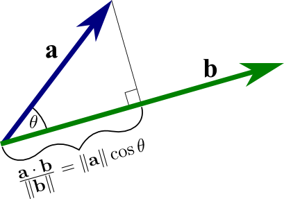
Fig. 73 Diagram of Scalar Projection and Dot Product. Image Credit: Math Insight#
Proof of Geometric Definition and The Law of Cosines#
For readers keen on proofs, the geometric definition of the dot product can be derived from the Law of Cosines.
Scalar projections#
Scalar projection offer a concise way to understand the geometric interpretation of the dot product by illustrating how one vector projects onto another. For the scalar projection of vector \(\mathbf{a}\) onto vector \(\mathbf{b}\), we are essentially looking at the length of the part of \(\mathbf{a}\) that aligns with the direction of \(\mathbf{b}\), assuming both vectors originate from the same point. This length, known as the scalar projection, can be positive, negative, or zero, reflecting the orientation of \(\mathbf{a}\) relative to \(\mathbf{b}\).
Mathematically, the scalar projection of \(\mathbf{a}\) onto \(\mathbf{b}\), denoted as \(\text{proj}_{\mathbf{b}} \mathbf{a}\), is given by:
where \(\mathbf{a} \cdot \mathbf{b}\) is the dot product of \(\mathbf{a}\) and \(\mathbf{b}\), and \(\|\mathbf{b}\|\) is the magnitude of \(\mathbf{b}\). This calculation reveals the component of \(\mathbf{a}\) that is in the same direction as \(\mathbf{b}\), providing a quantitative measure of how much \(\mathbf{a}\) ‘extends’ in the direction of \(\mathbf{b}\).
But how does this scalar projection relate to the dot product and the angle between the vectors? Here are a few key insights:
Measurement of Alignment: The scalar projection of vector \(\mathbf{a}\) onto vector \(\mathbf{b}\) quantifies the extent to which \(\mathbf{a}\) aligns along the direction of \(\mathbf{b}\). This alignment is crucial for understanding the dot product geometrically because the dot product, \(\mathbf{a} \cdot \mathbf{b} = \|\mathbf{a}\|\|\mathbf{b}\|\cos\theta\), essentially measures how much of \(\mathbf{a}\) lies in the direction of \(\mathbf{b}\) when considering the angle \(\theta\) between them. Scalar projection makes this concept tangible by providing a specific length value that represents this alignment.
Cosine of the Angle: The role of \(\cos\theta\) in the dot product formula is pivotal because it adjusts the magnitude of the product based on the angle between the two vectors. When \(\theta\) is small (vectors more aligned), \(\cos\theta\) is closer to 1, indicating a strong positive projection (i.e., \(\mathbf{a}\) largely points in the same direction as \(\mathbf{b}\)). When \(\theta\) is 90 degrees, \(\cos\theta\) is 0, reflecting orthogonal vectors with no projection onto each other. This relationship between \(\cos\theta\) and the scalar projection encapsulates the geometric interpretation of the dot product as a measure of vector alignment and interaction.
Understanding Vector Magnitudes and Direction: Scalar projections and the dot product together provide a comprehensive view of how vectors interact based not just on their direction but also on their magnitudes. The dot product takes into account both the size (magnitude) of the vectors and their directional relationship, offering a single scalar value that encapsulates both aspects. Through scalar projection, we see the practical application of these principles, where the magnitude of the projection tells us how much one vector extends in the direction of another, grounded in the vectors’ magnitudes and the angle between them.
Sign of the Dot Product is Determined by the Angle in between Two Vectors#
The geometric definition can be re-written as follows:
which essentially means that one can find the angle between two known vectors in any dimensional space.
The sign of the dot product is determined solely by the angle between the two vectors. By definition, \(\mathbf{a }\cdot\mathbf{b} = \|\mathbf{a}\|\ \|\mathbf{b}\|\cos\theta\), we know that the sign (positive or negative) of the dot product \(\mathbf{a} \cdot \mathbf{b}\) is solely determined by \(\cos \theta\) since \(\|\mathbf{a}\| \|\mathbf{b}\|\) is always positive.
Case 1 (\(0< \theta < 90\)): This implies that \(\cos \theta > 0 \implies \|\mathbf{a}\|\ \|\mathbf{b}\|\cos\theta > 0 \implies \mathbf{a}\cdot\mathbf{b} > 0\).
Case 2 (\(90 < \theta < 180\)): This implies that \(\cos \theta < 0 \implies \|\mathbf{a}\|\ \|\mathbf{b}\|\cos\theta < 0 \implies \mathbf{a}\cdot\mathbf{b} < 0\).
Case 3 (\(\theta = 90\)): This is an important property, for now, we just need to know that since \(\cos \theta = 0\), then \(\mathbf{a} \cdot \mathbf{b} = \mathbf{0}\). These two vectors are orthogonal.
Case 4 (\(\theta = 0\) or \(\theta = 180\)): This implies that \(\cos \theta = 1 \implies \|\mathbf{a}\|\ \|\mathbf{b}\|\cos\theta = \|\mathbf{a}\|\ \|\mathbf{b}\|\). We say these two vectors are collinear.
A simple consequence of case 4 is that if a vector \(\mathbf{a}\) dot product with itself, then by case 4, we have \(\mathbf{a} \cdot \mathbf{a} = \|\mathbf{a}\|^2 \implies \|\mathbf{a}\| = \sqrt{\mathbf{a} \cdot \mathbf{a}}\) which is the formula of the Euclidean length of the vector.
 1# Create plot with 4 subplots
 2fig, axes = plt.subplots(nrows=2, ncols=2, figsize=(20, 10))
 3
 4# Define common ax_kwargs for clarity and consistency
 5common_ax_kwargs = {
 6    "set_xlabel": {"xlabel": "x-axis", "fontsize": 16},
 7    "set_ylabel": {"ylabel": "y-axis", "fontsize": 16},
 8}
 9
10# Case 1: Acute angle
11plotter_case1 = VectorPlotter2D(
12    fig=fig,
13    ax=axes[0, 0],
14    ax_kwargs={
15        **common_ax_kwargs,
16        "set_xlim": {"left": -3, "right": 10},
17        "set_ylim": {"bottom": -3, "top": 10},
18        "set_title": {"label": "Case 1: $0< \\theta < 90$", "size": 18},
19    },
20)
21vectors_case1 = [
22    Vector2D(origin=(0, 0), direction=(4, 7), color="r", label="$\mathbf{u}$"),
23    Vector2D(origin=(0, 0), direction=(8, 4), color="b", label="$\mathbf{v}$"),
24]
25add_vectors_to_plotter(plotter_case1, vectors_case1)
26add_text_annotations(plotter_case1, vectors_case1)
27plotter_case1.plot()
28
29# Case 2: Obtuse angle
30plotter_case2 = VectorPlotter2D(
31    fig=fig,
32    ax=axes[0, 1],
33    ax_kwargs={
34        **common_ax_kwargs,
35        "set_xlim": {"left": -3, "right": 10},
36        "set_ylim": {"bottom": -3, "top": 10},
37        "set_title": {"label": "Case 2: $90 < \\theta < 180$", "size": 18},
38    },
39)
40vectors_case2 = [
41    Vector2D(origin=(0, 0), direction=(6, 2), color="r", label="$\mathbf{a}$"),
42    Vector2D(origin=(0, 0), direction=(-2, 4), color="b", label="$\mathbf{b}$"),
43]
44add_vectors_to_plotter(plotter_case2, vectors_case2)
45add_text_annotations(plotter_case2, vectors_case2)
46plotter_case2.plot()
47
48# Case 3: Orthogonal vectors
49plotter_case3 = VectorPlotter2D(
50    fig=fig,
51    ax=axes[1, 0],
52    ax_kwargs={
53        **common_ax_kwargs,
54        "set_xlim": {"left": -3, "right": 10},
55        "set_ylim": {"bottom": -3, "top": 10},
56        "set_title": {"label": "Case 3: $\\theta = 90$", "size": 18},
57    },
58)
59vectors_case3 = [
60    Vector2D(origin=(0, 0), direction=(6, 0), color="r", label="$\mathbf{a}$"),
61    Vector2D(origin=(0, 0), direction=(0, 6), color="b", label="$\mathbf{b}$"),
62]
63add_vectors_to_plotter(plotter_case3, vectors_case3)
64add_text_annotations(plotter_case3, vectors_case3)
65plotter_case3.plot()
66
67# Case 4: Collinear vectors
68plotter_case4 = VectorPlotter2D(
69    fig=fig,
70    ax=axes[1, 1],
71    ax_kwargs={
72        **common_ax_kwargs,
73        "set_xlim": {"left": -10, "right": 10},
74        "set_ylim": {"bottom": -3, "top": 10},
75        "set_title": {"label": "Case 4: $\\theta = 0$ or $\\theta = 180$", "size": 18},
76    },
77)
78vectors_case4 = [
79    Vector2D(origin=(0, 0), direction=(6, 0), color="r", label="$\mathbf{a}$"),
80    Vector2D(origin=(0, 0), direction=(-6, 0), color="b", label="$\mathbf{b}$"),
81]
82add_vectors_to_plotter(plotter_case4, vectors_case4)
83add_text_annotations(plotter_case4, vectors_case4)
84plotter_case4.plot()
85
86# Display the plot
87plt.tight_layout()
88plt.show()

Properties of Dot Product#
The dot product[1] fulfills the following properties if \(\mathbf{a}\), \(\mathbf{b}\), and \(\mathbf{c}\) are real vectors and \(\lambda\) is a scalar.
-
\(\mathbf{a} \cdot \mathbf{b} = \mathbf{b} \cdot \mathbf{a} ,\) which follows from the definition (\(\theta\) is the angle between a and b): \(\mathbf{a} \cdot \mathbf{b} = \left\| \mathbf{a} \right\| \left\| \mathbf{b} \right\| \cos \theta = \left\| \mathbf{b} \right\| \left\| \mathbf{a} \right\| \cos \theta = \mathbf{b} \cdot \mathbf{a} .\)
Distributive over vector addition:
\(\mathbf{a} \cdot (\mathbf{b} + \mathbf{c}) = \mathbf{a} \cdot \mathbf{b} + \mathbf{a} \cdot \mathbf{c} .\)
-
\(\mathbf{a} \cdot ( \lambda \mathbf{b} + \mathbf{c} ) = \lambda ( \mathbf{a} \cdot \mathbf{b} ) + ( \mathbf{a} \cdot \mathbf{c} ) .\)
-
\(( \lambda_1 \mathbf{a} ) \cdot ( \lambda_2 \mathbf{b} ) = \lambda_1 \lambda_2 ( \mathbf{a} \cdot \mathbf{b} ) .\)
Not associative:
This is because the dot product between a scalar value computed from \(\mathbf{a} \cdot \mathbf{b}\) and a vector \(\mathbf{c}\) is not defined, which means that the expressions involved in the associative property, \((\mathbf{a} \cdot \mathbf{b}) \cdot \mathbf{c}\) and \(\mathbf{a} \cdot (\mathbf{b} \cdot \mathbf{c})\), are both ill-defined. Note however that the previously mentioned scalar multiplication property is sometimes called the “associative law for scalar and dot product” or one can say that “the dot product is associative with respect to scalar multiplication” because \(\lambda (\mathbf{a} \cdot \mathbf{b}) = (\lambda \mathbf{a}) \cdot \mathbf{b} = \mathbf{a} \cdot (\lambda \mathbf{b})\).
-
Two non-zero vectors \(\mathbf{a}\) and \(\mathbf{b}\) are orthogonal if and only if \(\mathbf{a} \cdot \mathbf{b} = \mathbf{0}\).
No cancellation:
Unlike multiplication of ordinary numbers, where if \(ab=ac\) then b always equals c unless a is zero, the dot product does not obey the cancellation law.
-
If \(\mathbf{a}\) and \(\mathbf{b}\) are differentiable functions, then the derivative, denoted by a prime ‘ of \(\mathbf{a} \cdot \mathbf{b}\) is given by the rule \((\mathbf{a} \cdot \mathbf{b})' = \mathbf{a}' \cdot \mathbf{b} + \mathbf{a} \cdot \mathbf{b}'\).
Cauchy-Schwarz Inequality#
Let two vectors \(\mathbf{v}\) and \(\mathbf{w}\) be in a field \(\mathbb{F}^D\), then the inequality
holds.
This inequality establishes an upper bound for the dot product of two vectors, indicating that the absolute value of their dot product cannot exceed the multiplication of their individual norms. It’s important to note that this inequality reaches a point of equality only under two conditions: either both vectors are the zero vector \(\mathbf{0}\), or one vector is a scalar multiple of the other, denoted as \(\mathbf{v} = \lambda \mathbf{w}\). This principle underscores the inherent relationship between the geometric alignment of vectors and their magnitudes, providing a foundational concept in vector analysis and linear algebra.
The condition for equality, \(|\mathbf{v}^\top \mathbf{w}| = \|\mathbf{v}\| \|\mathbf{w}\|\), occurs precisely when \(\mathbf{v}\) and \(\mathbf{w}\) are linearly dependent, meaning one is a scalar multiple of the other (\(\mathbf{v} = \lambda \mathbf{w}\)). This situation represents vectors pointing in the same or exactly opposite directions, where their geometric alignment maximizes the dot product relative to their magnitudes. This specific case illustrates the tight bound provided by the inequality and its geometric interpretation as the projection of one vector onto another.
If you wonder why when \(\mathbf{v} = \lambda \mathbf{w}\) implies equality mathematically, it is apparent if you do a substitution as such
where we used the fact that \(\mathbf{w}^\top \mathbf{w} = \|\mathbf{w}\|^2\) by definition.
Proof of Algebraic and Geometric Equivalence of Dot Product#
For the sake of completeness, the proof of the equivalence of the algebraic and geometric definitions of the dot product can be found in ProofWiki.
Outer Product#
Definition#
Given two vectors of size \(m \times 1\) and \(n \times 1\) respectively
their outer product, denoted \(\mathbf{u} \otimes \mathbf{v}\) is defined as the \(m \times n\) matrix \(\mathbf{A}\) obtained by multiplying each element of \(\mathbf{u}\) by each element of \(\mathbf{v}\).
Or in index notation:
Denoting the dot product by \(\cdot\), if given an \(n \times 1\) vector \(\mathbf{w}\) then
If given a \(1 \times m\) vector \(\mathbf{x}\) then
If \(\mathbf{u}\) and \(\mathbf{v}\) are vectors of the same dimension, then \(\det (\mathbf{u} \otimes\mathbf{v}) = 0\).
The outer product \(\mathbf{u} \otimes \mathbf{v}\) is equivalent to a matrix multiplication \(\mathbf{u} \mathbf{v}^{\operatorname{T}}\) provided that \(\mathbf{u}\) is represented as a \(m \times 1\) column vector and \(\mathbf{v}\) as a \(n \times 1\) column vector (which makes \(\mathbf{v}^{\operatorname{T}}\) a row vector). For instance, if \(m = 4\) and \(n = 3,\) then
Column Wise Interpretation#
Especially from the matrix example in the previous section, one can see that the following holds:
What this means is that in our example our column vector is \(\mathbf{u}\). Then when we do an outer product of \(\mathbf{u}\) on \(\mathbf{v}\), then notice each of the resultant matrix’s columns is a scaled version of the column vector \(\mathbf{u}\), scaled none other by the elements of the row vector \(\mathbf{v}\) itself.
Row Wise Interpretation#
Especially from the matrix example in the previous section, one can see that the following holds:
What this means is that in our example our row vector is \(\mathbf{v}\). Then when we do an outer product of \(\mathbf{u}\) on \(\mathbf{v}\), then notice each of the resultant matrix’s rows is a scaled version of the row vector \(\mathbf{v}\), scaled none other by the elements of the row vector \(\mathbf{u}\) itself.
Transpose Property#
\(\mathbf{u}\mathbf{v}^\top\) and \(\mathbf{v}\mathbf{u}^\top\). What can you deduce from this? Actually if you do an example, you will notice that the resulting matrices are the same with rows and columns swapped. That is,
References and Further Readings#
Geometrical meanings of a dot product and cross product of a vector - Quora
What does the dot product of two vectors represent - Math Stack Exchange