Vector Norm and Distance#
We first start off by mentioning that we will revisit this section later in the series in a more rigorous manner. For now, we will have a first look on the naive interpretation of vector norms and distances.
Understanding the norm of a vector is fundamental in various fields, including machine learning, where it is crucial for tasks like normalizing data, measuring similarity, and regularization. In the context of generative AI and embedding spaces, norms play an important role in quantifying the magnitude and distance of vectors, which represent complex entities like features, words, or even images.
Norm#
We start off with the formal definition of a norm. We will also define \(\mathbf{v}\) as a vector in \(\mathbb{R}^D\), where \(D\) is the dimension of the vector space:
Definition 38 (Norm on a Vector Space)
A norm on a vector space \(\mathcal{V}\) over a field \(\mathbb{F}\) (typically \(\mathbb{R}\) or \(\mathbb{C}\)), is a function
which assigns each vector \(\mathbf{v} \in \mathcal{V}\) a real number \(\|\mathbf{v}\|\), representing the length of \(\mathbf{v}\) [Deisenroth et al., 2020].
This function must satisfy the following properties for all scalars \(\lambda\) and vectors \(\mathbf{u}, \mathbf{v} \in \mathcal{V}\):
Absolute Homogeneity (or Positive Scaling):
\[ \|\lambda \mathbf{u}\| = |\lambda| \|\mathbf{u}\| \]This means the norm is scale-invariant and respects scalar multiplication.
Triangle Inequality:
\[ \|\mathbf{u} + \mathbf{v}\| \leq \|\mathbf{u}\| + \|\mathbf{v}\| \]The sum of the norms of two vectors is always greater than or equal to the norm of their sum.
Positive Definiteness:
\[ \|\mathbf{u}\| \geq 0 \text{ and } \|\mathbf{u}\| = 0 \iff \mathbf{u} = \mathbf{0} \]The norm of any vector is non-negative and is zero if and only if the vector itself is the zero vector.
We are being ahead of ourselves because we did not define what is a vector space. We will revisit this later in the series. For now, treat a vector space as a set of vectors in the \(D\)-dimensional space \(\mathbb{R}^D\).
\(L^{p}\) Norm#
With the norm well defined, we can now define the \(L_p\) norm, which is a specific case of the norm function. The \(L_p\) is a generalization of the concept of “length” for vectors in the vector space \(\mathcal{V}\).
Definition 39 (\(L_p\) Norm)
For a vector space \(\mathcal{V} = \mathbb{R}^D\) over the field \(\mathbb{F} = \mathbb{R}\), the \(L_p\) norm is a function defined as:
where each vector \(\mathbf{v} \in \mathcal{V}\) (defined as in (20)) is assigned a real number \(\|\mathbf{v}\|_p\), representing the \(L_p\) norm of \(\mathbf{v}\).
In other words, for a vector \(\mathbf{v} \in \mathbb{R}^D\), the \(L_p\) norm of \(\mathbf{v}\), denoted as \(\|\mathbf{v}\|_p\), is defined as:
where \(v_1, v_2, \ldots, v_D\) are the components of the vector \(\mathbf{v}\), and \(p\) is a real number greater than or equal to 1.
One can easily verify that the \(L_p\) norm satisfies the properties of a norm function in Definition 38.
As we shall see later (likely when we discuss about analytic geometry), the choice of \(p\) determines the metric’s sensitivity to differences in vector components, influencing its application in various algorithms.
\(L_1\) Norm (Manhattan Norm)#
The \(L_1\) norm, also known as the Manhattan norm or Taxicab norm, is a specific case of the \(L_p\) norm where \(p = 1\).
Definition 40 (\(L_1\) Norm)
For the same vector space \(\mathcal{V} = \mathbb{R}^D\), the \(L_1\) norm is defined by:
assigning to each vector \(\mathbf{v}\) (defined as in (20)) the sum of the absolute values of its components, \(\|\mathbf{v}\|_1\).
In other words, for a vector \(\mathbf{v} \in \mathbb{R}^D\), the \(L_1\) norm of \(\mathbf{v}\), denoted as \(\|\mathbf{v}\|_1\), is defined as:
This norm is called the Manhattan norm because it is the distance between two points in a grid-like Manhattan street layout, where the shortest path between two points is the sum of the horizontal and vertical distances. This metric sums the absolute values of the vector components. Geometrically, it measures the distance a taxicab (hence the name taxicab) would travel in a grid-like path in \(\mathbb{R}^D\). In machine learning, the \(L_1\) norm is often used for regularization, encouraging sparsity in the model parameters.
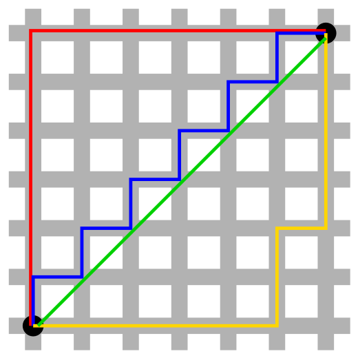
Fig. 16 Taxicab geometry versus Euclidean distance: In taxicab geometry, the red, yellow, and blue paths all have the same length of 12. In Euclidean geometry, the green line has length \(6 \sqrt{2} \approx 8.49\) and is the unique shortest path, while the other paths have the longer length of 12.#
Image Credit: Wikipedia
\(L_2\) Norm (Euclidean Norm)#
The \(L_2\) norm, or Euclidean norm, obtained by setting \(p = 2\), is the most familiar norm in machine learning.
Definition 41 (L2 Norm)
Similarly, for \(\mathcal{V} = \mathbb{R}^D\), the \(L_2\) norm is given by:
where \(\|\mathbf{v}\|_2\) is the Euclidean length of the vector \(\mathbf{v}\) (defined as in (20)).
In other words, for a vector \(\mathbf{v} \in \mathbb{R}^D\), the \(L_2\) norm of \(\mathbf{v}\), denoted as \(\|\mathbf{v}\|_2\), is defined as:
It measures the “straight-line” distance from the origin to the point in \(\mathbb{R}^D\) represented by \(\mathbf{v}\). This norm is extensively used in machine learning to measure the magnitude of vectors, in optimization algorithms (like gradient descent), and in computing distances between points in feature space.
With reference to figure Fig. 16, the green line defines the Euclidean distance between two points in \(\mathbb{R}^2\) and is the shortest path between the two points.
Let’s see how the L2 norm looks like in a 2D space.
Show code cell source
 1fig, ax = plt.subplots(figsize=(9, 9))
 2
 3plotter = VectorPlotter2D(
 4    fig=fig,
 5    ax=ax,
 6    ax_kwargs={
 7        "set_xlim": {"left": 0, "right": 5},
 8        "set_ylim": {"bottom": 0, "top": 5},
 9        "set_xlabel": {"xlabel": "x-axis", "fontsize": 16},
10        "set_ylabel": {"ylabel": "y-axis", "fontsize": 16},
11        "set_title": {"label": "Vector Magnitude Demonstration", "size": 18},
12    },
13)
14
15v = Vector2D(
16    origin=(0, 0),
17    direction=(3, 4),
18    color="r",
19    label="$\|\mathbf{v}\|_2 = \sqrt{3^2 + 4^2} = 5$",
20)
21horizontal_component_v = Vector2D(
22    origin=(0, 0), direction=(3, 0), color="b", label="$v_1 = 3$"
23)
24vertical_component_v = Vector2D(
25    origin=(3, 0), direction=(0, 4), color="g", label="$v_2 = 4$"
26)
27add_vectors_to_plotter(plotter, [v, horizontal_component_v, vertical_component_v])
28add_text_annotations(plotter, [v])
29
30plotter.plot()

Notice that the calculation is equivalent to the Pythagorean theorem, where the length of the hypotenuse is the square root of the sum of the squares of the other two sides.
We can easily calculate the L2 norm of a vector using NumPy:
1u = np.array([3, 4])
2rich.print(f"Norm of u: {np.linalg.norm(u)}")
Norm of u: 5.0
And as convenience, our vector object v has an property/attribute l2_norm
(magnitude) that returns the L2 norm of the vector.
1v = Vector2D(
2    origin=(0, 0),
3    direction=(3, 4),
4    color="r",
5    label="$\|\mathbf{v}\|_2 = \sqrt{3^2 + 4^2} = 5$",
6)
7rich.print(f"Norm of v: {v.l2_norm}")
Norm of v: 5.0
Generalization of the Pythagorean Theorem to \(D\) Dimensions#
The Pythagorean theorem generalizes to \(D\) dimensions, where the length of the hypotenuse is the square root of the sum of the squares of the other sides.
We can use 3D as a way to illustrate this. The following series of images are taken from Math is Fun.
First, consider Fig. 17, we want to find the length of the diagonal.

Fig. 17 Finding the length of the diagonal.#
Image Credit: Math is Fun
We can first use Pythagorean theorem to find the length of the diagonal of the base.
where \(c\) is the length of the diagonal of the base.

Fig. 18 Image Credit: Math is Fun#
Then, the diagonal base serves as one of the sides of the triangle that we want to find.

Fig. 19 Image Credit: Math is Fun#
Finally, we use Pythagorean theorem again to find the length of the diagonal.

Fig. 20 The Pythagorean Theorem in 3D.#
Image Credit: Math is Fun
Without loss of generality (we are being less pedantic here), we can generalize the Pythagorean theorem to \(D\) dimensions, illustrated in Table 22 below.
We denote \(d\) as the length of the diagonal, and \(a_1, a_2, \ldots, a_D\) as the length of the sides of the triangle (or the vector components).
Dimension |
Pythagoras |
Distance/Norm |
|---|---|---|
1 |
\(d^2 = a_1^2\) |
\(d = \sqrt{a_1^2} = \|a\|_2\) |
2 |
\(d^2 = a_1^2 + a_2^2\) |
\(d = \sqrt{a_1^2 + a_2^2} = \|a\|_2\) |
3 |
\(d^2 = a_1^2 + a_2^2 + a_3^2\) |
\(d = \sqrt{a_1^2 + a_2^2 + a_3^2} = \|a\|_2\) |
… |
… |
… |
\(D\) |
\(d^2 = a_1^2 + a_2^2 + \cdots + a_D^2\) |
\(d = \sqrt{a_1^2 + a_2^2 + \cdots + a_D^2} = \|a\|_2\) |
Distance#
We have been using distance and norm interchangeably. However, they are not exactly the same.
The key difference (without going to deep into real analysis and metric spaces) is that the norm as defined in Definition 38 is a function that maps a vector to a field \(\mathbb{F}\) (i.e. real number \(\mathbb{R}\)), while the distance is a function that maps a pair of vectors to a field \(\mathbb{F}\).
Definition 42 (Distance)
A distance on a vector space \(\mathcal{V}\) over a field \(\mathbb{F}\) (typically \(\mathbb{R}\) or \(\mathbb{C}\)), is a function
which assigns each pair of vectors \(\mathbf{u}, \mathbf{v} \in \mathcal{V}\) a real number \(d(\mathbf{u}, \mathbf{v})\), representing the distance between \(\mathbf{u}\) and \(\mathbf{v}\). This function must satisfy the following properties for all vectors \(\mathbf{u}, \mathbf{v}, \mathbf{w} \in \mathcal{V}\) [Muscat, 2014]:
Non-negativity:
\[ d(\mathbf{u}, \mathbf{v}) \geq 0 \]The distance between any two vectors is non-negative.
Identity of Indiscernibles:
\[ d(\mathbf{u}, \mathbf{v}) = 0 \iff \mathbf{u} = \mathbf{v} \]The distance between two vectors is zero if and only if the vectors are identical.
Symmetry:
\[ d(\mathbf{u}, \mathbf{v}) = d(\mathbf{v}, \mathbf{u}) \]The distance between two vectors is the same regardless of the order of the vectors.
Triangle Inequality:
\[ d(\mathbf{u}, \mathbf{v}) \leq d(\mathbf{u}, \mathbf{w}) + d(\mathbf{w}, \mathbf{v}) \]The distance between two vectors is always less than or equal to the sum of the distances between the vectors and a third vector.
We say that every norm induces a distance metric defined in Definition 42.
Why?
Given a norm \(\|\cdot\|\) on a vector space \(\mathcal{V}\), one can define a distance function induced by this norm as \(d(\mathbf{u}, \mathbf{v})=\|\mathbf{u}-\mathbf{v}\|\) for all \(\mathbf{u}, \mathbf{v} \in \mathcal{V}\). This distance function satisfies the metric space properties:
Non-negativity: For any vectors \(\mathbf{u}, \mathbf{v}\), the distance \(d(\mathbf{u}, \mathbf{v})\) is never negative because norms are always non-negative. This is a direct result of the norm’s property of positive definiteness (Definition 38).
Identity of Indiscernibles: The distance \(d(\mathbf{u}, \mathbf{v})\) is zero if and only if \(\mathbf{u} = \mathbf{v}\). This follows from the positive definiteness property (Definition 38) of norms which states that \(\|\mathbf{u}\| = 0\) if and only if \(\mathbf{u} = \mathbf{0}\). Thus, \(\|\mathbf{u} - \mathbf{v}\| = 0\) implies \(\mathbf{u} - \mathbf{v} = \mathbf{0}\), which means \(\mathbf{u} = \mathbf{v}\).
Symmetry: The distance function is symmetric, meaning \(d(\mathbf{u}, \mathbf{v}) = d(\mathbf{v}, \mathbf{u})\) for all \(\mathbf{u}, \mathbf{v}\). This is because \(\|\mathbf{u}-\mathbf{v}\| = \|\mathbf{v}-\mathbf{u}\|\), as the norm of a vector remains the same if its sign is reversed. This follows directly from the norm’s property of absolute homogeneity (Definition 38) because you can just set \(\lambda = -1\). Thus, \(\|\mathbf{u}-\mathbf{v}\| = \|-1\| \|\mathbf{v}-\mathbf{u}\| = \|\mathbf{v}-\mathbf{u}\|\).
Triangle Inequality: The distance satisfies the triangle inequality, which states that for any \(\mathbf{u}, \mathbf{v}, \mathbf{w} \in \mathcal{V}\), the inequality \(d(\mathbf{u}, \mathbf{w}) \leq d(\mathbf{u}, \mathbf{v}) + d(\mathbf{v}, \mathbf{w})\) holds. This is a consequence of the norm’s triangle inequality (Definition 38), \(\|\mathbf{u}+\mathbf{v}\| \leq \|\mathbf{u}\| + \|\mathbf{v}\|\), applied to the vectors \(\mathbf{u}-\mathbf{v}\) and \(\mathbf{v}-\mathbf{w}\), which yields \(\|\mathbf{u}-\mathbf{w}\| \leq \|\mathbf{u}-\mathbf{v}\| + \|\mathbf{v}-\mathbf{w}\|\).
Thus, the norm-induced distance function \(d\) adheres to all the axioms of a metric and therefore defines a metric space on \(\mathcal{V}\). This provides a way to measure “distances” in vector spaces that are consistent with the structure and properties of the space as defined by the norm.
For example, the \(L_2\) norm \(\|\cdot\|_2\) induces the Euclidean distance \(d(\mathbf{u}, \mathbf{v}) = \|\mathbf{u}-\mathbf{v}\|_2\) between two vectors \(\mathbf{u}, \mathbf{v} \in \mathbb{R}^D\). The key to remember that the transition of a norm to a distance is the subtraction of two vectors. So the domain of the distance function is a pair of vectors, while the domain of the norm function is a single vector. There is no confusion because \(d(\mathbf{u}, \mathbf{v})\) indeed takes in two vectors as input, while the right hand side of the equation \(\|\mathbf{u}-\mathbf{v}\|_2\) is a single vector.
Furthermore, the \(L_2\) norm of a single vector \(\mathbf{v}\) is equivalent to the Euclidean distance between \(\mathbf{v}\) and the origin \(\mathbf{0}\), and the \(L_2\) norm of the difference between two vectors \(\mathbf{u}\) and \(\mathbf{v}\) is equivalent to the Euclidean distance between \(\mathbf{u}\) and \(\mathbf{v}\). Therefore, we often use the term “norm” and “distance” interchangeably because if we set the component \(\mathbf{v} = \mathbf{0}\), then we recover the norm of \(\mathbf{u}\).
It is important to note that while norms always induce a metric, not all metrics arise from norms. A metric that does not come from a norm might not satisfy the properties of homogeneity or the triangle inequality in the same way that a norm does.
For such distances, while they may satisfy the properties required of a metric, they cannot be expressed as the norm of the difference between two vectors. Two examples are given:
The discrete metric:
\[\begin{split} d(x, y)= \begin{cases}0 & \text { if } x=y \\ 1 & \text { if } x \neq y\end{cases} \end{split}\]The arctangent metric on \(\mathbb{R}\):
\[ d(x, y)=|\arctan (x)-\arctan (y)| \]
Both of these satisfy the properties of a metric but are not induced by any norm because they do not satisfy the homogeneity property (scaling) and, in the case of the discrete metric, do not satisfy the triangle inequality as it would be defined by a norm.
Closing: Relevance of Vector Norms and Distances in Machine Learning and Deep Learning#
The concepts of vector norms and distances, as explored previously, play a crucial role in the realms of machine learning and deep learning. Their relevance can be highlighted in several key aspects of these fields:
Feature Normalization: In many machine learning algorithms, it’s important to normalize or scale features so that they contribute equally to the learning process. Vector norms, especially the \(L_2\) norm, are often used to normalize data, ensuring that each feature contributes proportionately to the overall model.
Similarity and Distance Metrics: In clustering algorithms like K-means or in nearest neighbor searches, the notion of distance between data points is fundamental. Here, norms (like the Euclidean or Manhattan norms) define the metrics used to quantify the similarity or dissimilarity between points in the feature space.
Regularization in Optimization: In both machine and deep learning, regularization techniques are employed to prevent overfitting. The \(L_1\) (Lasso) and \(L_2\) (Ridge) norms are particularly notable for their use in regularization terms. \(L_1\) regularization encourages sparsity in the model parameters, which can be beneficial for feature selection, while \( L_2\) regularization penalizes large weights, promoting smoother solution spaces.
Embedding Spaces in Deep Learning: In deep learning, particularly in areas like natural language processing or image recognition, the concept of embedding spaces is vital. These are high-dimensional spaces where similar items are placed closer together. Norms and distances in these spaces are used to measure the closeness or similarity of different entities (like words, sentences, or images), impacting the performance of models like neural networks.
Gradient Descent and Backpropagation: The core of training deep learning models involves optimization techniques like gradient descent. The \( L_2\) norm is particularly important in quantifying the magnitude of gradients, guiding the update steps in the learning process.
Loss Functions: Many machine learning models are trained by minimizing a loss function. The choice of this function often involves norms and distances. For instance, mean squared error (a common loss function) is essentially an \(L_2\) norm of the error vector.
Autoencoders in Deep Learning: Autoencoders, used for dimensionality reduction or feature learning, often utilize norms to measure the reconstruction loss, i.e., the difference between the input and its reconstruction.
Anomaly Detection: In anomaly detection, distances from a norm or a threshold often signify whether a data point is an anomaly or not.
In conclusion, vector norms and distances are not just abstract mathematical concepts; they are tools deeply ingrained in the fabric of machine learning and deep learning. They provide the means to measure, compare, and optimize in the multi-dimensional spaces that these fields operate in, making them indispensable in the toolkit of anyone working in these domains.
This is by no means we will deal with norms and distances. We will revisit this when we discuss about analytic geometry - which spans concepts such as similarity, inner product, orthogonality, and projections.
References and Further Readings#
Deisenroth, M. P., Faisal, A. A., & Ong, C. S. (2020). Mathematics for Machine Learning. Cambridge University Press. (Chapter 3.1, Norms).
Muscat, J. Functional Analysis An Introduction to Metric Spaces, Hilbert Spaces, and Banach Algebras, Springer, 2014.