The Concept of Generative Pre-trained Transformers (GPT)#
Motivation#
The problem that GPT-2 aims to solve is to demonstrate that language models, given large enough capacity in terms of parameters, and large enough unlabeled and high-quality text data, can solve specialized natural language processing tasks such as question answering, translation, and summarization, in a zero-shot manner - without the need for task-specific architectures or supervised fine-tuning.
The emphasis on the large and high-quality text data cannot be understated as the authors are hinging on the fact that the dataset is so diverse, and therefore bound to have examples of the specialized tasks that the model can learn from.
For example, if we are looking at translation tasks, then the data is bound to have somewhat sequential and natural occuring translation text such as:
The translation of the french sentence 'As-tu aller au cine ́ma?' to english is 'Did you go to the cinema?'.
The model can learn from such examples and generalize to perform well on the translation task via the autoregressive, self-supervised learning paradigm without the need for supervised fine-tuning.
From GPT-1 to GPT-2#
In Natural Language Understanding (NLU), there are a wide range of tasks, such as textual entailment, question answering, semantic similarity assessment, and document classification. These tasks are inherently labeled, but given the scarcity of such data, it makes discriminative models such as Bidirectional Long Short-Term Memory (Bi-LSTM) underperform [Radford et al., 2018], leading to poor performance on these tasks.
In the GPT-1 paper Improving Language Understanding by Generative Pre-Training, the authors demonstrated that generative pre-training of a language model on a diverse corpus of unlabeled text, followed by discriminative fine-tuning on each specific task, can overcome the constraints of the small amount of annotated data for these specific tasks. The process is collectively termed as semi-supervised learning and the goal is to learn an universal representation of the natural language space that can be used across a wide range of tasks.
The pretraining objective is to predict the next token in a sequence, in an autoregressive manner, given the previous tokens. The pretrained model, often known as the foundational model (or backbone), serves as a base from which specialized capabilities can be added through fine-tuning on specific tasks. In the fine-tuning phase, task-specific adaptations are necessary: the input format must be adjusted to align with the particular requirements of the task at hand, and the model’s final layer—or “head”—needs to be replaced to accommodate the task’s specific class structure. The author showed that this approach yielded state-of-the-art results on a wide range of NLU tasks.
Notwithstanding the success of this approach, the same set of authors came up with a new paper in the following year, titled Language Models are Unsupervised Multitask Learners, where they introduced a new model, GPT-2, that was larger in model capacity, and trained on a much larger unlabeled corpus, WebText. However, the key innovation was to void the supervised fine-tuning step, and instead, they demonstrated that GPT-2 could be used directly on a wide range of NLU tasks directly, with what they termed as the zero-shot transfer. The motivation is that the authors think that foundational language models should be competent generalists, rather than narrowly experts [Radford et al., 2019]. They call for the need to shift the language model paradigm to one that is generic enough to handle NLU tasks without the need to curate specific training data for each specific task.
In what follows, we would first review the key concepts and ideas of the GPT-2 paper, formalize the autoregressive self-supervised learning paradigm, and then take a look at the implementation of the GPT-2 model.
GPT-2 Paper Key Ideas#
In this section, we would review the key ideas from the GPT-2 paper.
Abstract Overview#
Below are the key ideas from the abstract of the GPT-2 paper:
All previous pretrained language models necessitated a secondary stage of supervised fine-tuning to tailor them to specific downstream tasks.
The authors showcased that, given sufficient model capacity and data, language models can be adeptly adjusted to a broad spectrum of tasks without the need for task-specific architectural modifications.
When tasked with a question-answering challenge, specifically conditioned on a document and questions using the CoQA dataset — comprised of over 127,700 training examples — the model demonstrates the capability to match or surpass the performance of three baseline models.
An emphasis is placed on the model’s capacity as being integral to the success of zero-shot transfer. It’s highlighted that the model’s performance escalates in a log-linear fashion relative to the number of parameters, signifying that as the model’s capacity increases logarithmically, its performance improves linearly.
Introduction#
In this section, we would discuss the key ideas from the introduction of the GPT-2 paper.
Key 1. Competent Generalists over Narrow Experts (1)#
The authors cited other works that have demonstrated significant success of machine learning systems through a combination of large-scale data, high model capacity, along with supervised fine-tuning.
However, such systems, termed as “narrow experts,” are fragile, as they are highly dependent on the specific training regime and task. A slight perturbation to the input distribution can cause the model to perform poorly.
The authors then expressed the desire for “competent generalists” that can perform well across a wide range of tasks without the need for task-specific architectures or supervised fine-tuning.
Key 2. IID Assumption Fails in Real World (2, 3)#
The overarching goal in machine learning is to generalize to unseen data points. To streamline the modeling of machine learning objectives, it’s commonly assumed that the training and test data are drawn from the same distribution, a concept known as the Independent and Identically Distributed (i.i.d.) assumption.
As an aside, the i.i.d. assumption is foundational in statistical modeling because it simplifies the process significantly. For example, it allows us to express joint probability distributions as the product of marginal distributions.
Furthermore, evaluation techniques such as resampling and cross-validation with a holdout set rely on the assumption that the training and test data are drawn from the same distribution.
However, as the authors highlighted, the i.i.d. assumption fails in the real world. The distribution of the test data is often different from the training data, and the model’s performance degrades significantly when the test data distribution is different from the training data distribution.
They attribute this to the prevalence of single task training on single domain datasets, which limits the model’s ability to generalize across diverse conditions and tasks.
Key 3. Multi-Task Learning is Nacent (4)#
The author then underscored that multi-task learning represents a promising framework. By training a single model on multiple tasks simultaneously, the model is enabled to leverage generalizable latent space embeddings and representations to excel across various tasks.
It was further pointed out that recent work in the field utilizes, for example, 10 (dataset, objective) pairs [McCann et al., 2018] to train a singular model (an approach known as meta-learning). This implies that:
Each dataset and its corresponding objective are unique.
For instance, one dataset might focus on sentiment data, with the goal of predicting sentence sentiment, whereas another dataset might concentrate on named entity recognition, aiming to identify named entities within a sentence.
The challenge then circles back to the compilation, curation, and annotation of these datasets and objectives to ensure the model’s generalizability. Essentially, this dilemma mirrors the initial issue of single-task training on single-domain datasets. The implication is that training a multi-task model might require an equivalent volume of curated data as training several single-task models. Furthermore, scalability becomes a concern when the focus is limited to merely 10 (dataset, objective) pairs.
Key 4. From Word Embeddings to Contextual Embeddings (5,6)#
Initially, word embeddings such as Word2Vec and GloVe revolutionized the representation of words by mapping them into dense, fixed-dimensional vectors within a continuous \(D\) dimensional space, hinging on the fact that words occuring in similar contexts/documents are similar semantically. These vectors were then used as input to a model to perform a specific task.
The next advancement is capturing more contextual information by using contextual embeddings, where the word embeddings are conditioned on the entire context of the sentence. Recurrent Neural Networks (RNNs) is one example and the context embeddings can be “transferred” to other downstream tasks.
Specifically, unidirectional RNNs are adept at assimilating context from preceding elements, whereas bidirectional RNNs excel in integrating context from both preceding and succeeding elements. Nonetheless, both strategies grapple with challenges in encoding long-range dependencies.
Moreover, RNNs are notoriously plagued by the gradient vanishing problem, which means that the model is biased by the most recent tokens in the sequence, and the model’s performance degrades as the sequence length increases.
Self-attention mechanisms, foundational to the Transformer architecture, mark a paradigm shift by enabling each token to “attend” to every other token within a sequence concurrently.
This allows the model to capture long-range dependencies and is the basis for the Transformer architecture. Consequently, self-attention is non-sequential by design and operates over a set of tokens, and not a sequence of tokens. This calls for the need to introduce positional encodings to the input embeddings to capture the sequential nature of the tokens.
This advancement transcends the limitations of static word embeddings. Now, given two sentences, I went to the river bank versus i went to the bank to withdraw money, the word “bank” in the first sentence is semantically different from the word “bank” in the second sentence. The contextual embeddings can capture this difference.
The authors then went on to mention that the above methods would still require supervised fine-tuning to adapt to a specific task.
If there are minimal or no supervised data is available, there are other lines of work using language model to handle it - commonsense reasoning (Schwartz et al., 2017) and sentiment analysis (Radford et al., 2017).
Key 5. Zero Shot Learning and Zero Shot Transfer (7)#
Building upon the foundational concepts introduced previously, the authors explore the utilization of general methods of transfer to illustrate how language models can adeptly execute downstream tasks in a zero-shot manner, without necessitating any modifications to parameters or architecture.
Zero-shot learning (ZSL) is characterized by a model’s capability to accurately execute tasks or recognize categories that it was not explicitly trained to handle. The crux of ZSL lies in its ability to generalize from known to unknown classes or tasks by harnessing side information or semantic relationships.
For example, a model trained to recognize on a set of animals (including horses) but not on zebra, should be able to recognize a zebra as something close to horse, given the semantic relationship between the two animals.
Zero-shot transfer, often discussed within the context of transfer learning, involves applying a model trained on one set of tasks or domains to a completely new task or domain without any additional training. Here, the focus is on the transferability of learned features or knowledge across different but related tasks or domains. Zero-shot transfer extends the concept of transfer learning by not requiring any examples from the target domain during training, relying instead on the model’s ability to generalize across different contexts based on its pre-existing knowledge.
Section 2. Approach#
In this section, we would discuss the key ideas from the approach section of the GPT-2 paper.
Key 1. Modeling Language Models over Joint Probability Distributions (1)#
Language models strive to approximate the complex and inherently unknown distribution of the natural language space, denoted as \(\mathcal{D}\). In contrast to supervised learning, which explicitly separates inputs (\(\mathcal{X}\)) from labels (\(\mathcal{Y}\)), unsupervised learning — particularly when employing self-supervision as seen in language modeling — blurs this distinction. Here, \(\mathcal{Y}\) is conceptually a shifted counterpart of \(\mathcal{X}\), facilitating a unified approach where \(\mathcal{D}\) can be modeled exclusively over the space of \(\mathcal{X}\). This scenario allows us to frame \(\mathcal{D}\) as a probability distribution across sequences of tokens within \(\mathcal{X}\), parameterized by \(\boldsymbol{\Theta}\).
In this context, the essence of language modeling is to characterize the joint probability distribution of sequences \(\mathbf{x} = (x_1, x_2, \ldots, x_T)\) within \(\mathcal{X}\). The goal is to maximize the likelihood of observing these sequences in a corpus \(\mathcal{S}\), denoted as \(\hat{\mathcal{L}}(\mathcal{S} ; \hat{\boldsymbol{\Theta}})\), where \(\hat{\boldsymbol{\Theta}}\) represents the estimated parameter space that approximates the true parameter space \(\boldsymbol{\Theta}\).
Key 2. Decompose Joint Distributions as Conditional Distributions via Chain Rule (2)#
The joint probability of a sequence in natural language, inherently ordered [Radford et al., 2019], can be factorized into the product of conditional probabilities of each token in the sequence using the chain rule of probability. This approach not only enables tractable sampling from and estimation of the distribution \(\mathbb{P}(\mathbf{x} ; \boldsymbol{\Theta})\) but also facilitates modeling conditionals in forms such as \(\mathbb{P}(x_{t-k} \ldots x_t \mid x_1 \ldots x_{t-k-1} ; \boldsymbol{\Theta})\) [Radford et al., 2019]. Given a corpus \(\mathcal{S}\) with \(N\) sequences, the likelihood function \(\hat{\mathcal{L}}(\mathcal{S} ; \hat{\boldsymbol{\Theta}})\) represents the likelihood of observing these sequences. The ultimate objective is to maximize this likelihood, effectively approximating the joint probability distribution through conditional probability distributions.
Key 3. Conditional on Task (3)#
In the GPT-2 paper, Language Models are Unsupervised Multitask Learners, the authors introduced the concept of conditional on task where the GPT model \(\mathcal{G}\) theoretically should not only learn the conditional probability distribution \(\mathbb{P}(x_t \mid x_{<t} ; \boldsymbol{\Theta})\) but also learn the conditional probability distribution \(\mathbb{P}(x_t \mid x_{<t} ; \boldsymbol{\Theta}, \mathcal{T})\) where \(\mathcal{T}\) is the task that the model should implicitly learn [Radford et al., 2019]. This is a powerful concept because if such a hypothesis is correct, then the GPT model \(\mathcal{G}\) can indeed be a multi-task learner, and can be used directly on a wide range of NLU tasks without the need for supervised fine-tuning for downstream domain-specific tasks.
In practice, the authors mentioned that task conditioning is often implemented at an architectural level, via task specific encoder and decoder in the paper One Model To Learn Them All [Kaiser et al., 2017], for instance, or at an algorithmic level, such as the inner and outer loop optimization framework, as seen in the paper Model-Agnostic Meta-Learning for Fast Adaptation of Deep Networks [Finn et al., 2017].
However, the authors further mentioned that without task-specific architectural
changes, one can leverage the sequential nature of the natural language space
where we can construct a tasks, inputs and outputs all as a sequence of symbols
[Radford et al., 2019]. For example, a translation task can be formulated
as a sequence of symbols via
(translate to french, english sequence, french sequence), where the model can
now learn to also condition on the task (translate to french) in addition to
the sequence of tokens. The paper The Natural Language Decathlon: Multitask
Learning as Question Answering exemplifies this concept with their model
Multitask Question Answering Network (MQAN), where a single model is trained
to perform many diverse natural language processing tasks simultaneously.
Key 4. Optimizing Unsupervised is the same as Optimizing Supervised (4)#
The GPT-2 paper Language Models are Unsupervised Multitask Learners demonstrated that they want to do away with the supervised fine-tuning phase via an interesting hypothesis, that optimizing the unsupervised objective is the same as optimizing the supervised objective because the global minimum of the unsupervised objective is the same as the global minimum of the supervised objective [Radford et al., 2019].
Key 5. Large Language Models has Capacity to Infer and Generalize (5)#
In what follows, the author added that the internet contains a vast amount of information that is passively available without the need for interactive communication. The example that I provided on the french-to-english translation would bound to exist naturally in the internet. They speculate that if the language model is large enough in terms of capacity, then it should be able to learn to perform the tasks demonstrated in natural language sequences in order to better predict them, regardless of their method of procurement [Radford et al., 2019].
In the figure below, we can see examples of naturally occurring demonstrations of English to French and French to English translation found throughout the WebText training set.
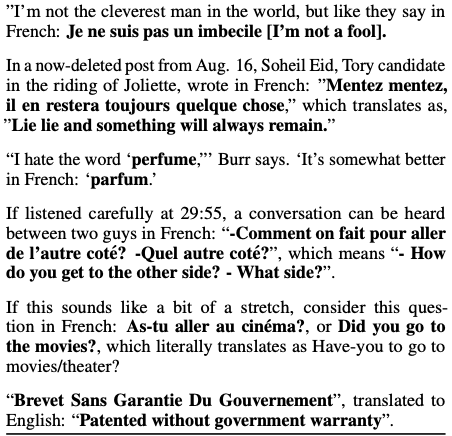
Fig. 1 Examples of naturally occurring demonstrations of English to French and French to English translation found throughout the WebText training set.#
Image Credit: Language Models are Unsupervised Multitask Learners
2.1. Training Dataset#
Key 1. Rejection of CommonCrawl (1,2)#
Prior research often focused on training language models on single-domain datasets, which relates to the concept of models becoming narrow experts.
To cultivate competent generalists, the authors contend that models need exposure to a diverse array of tasks and domains.
CommonCrawl, housing an expansive collection of web scrapes (essentially capturing the entirety of the internet), is recognized for its diversity.
Nevertheless, CommonCrawl was ultimately rejected by the authors due to significant data quality issues.
Key 2. Construction of WebText Dataset#
The authors sought to compile a web scrape prioritizing document quality over quantity.
To attain a certain level of document quality without the exorbitant costs of manual curation, the authors employed a strategy of indirect human curation. This involved scraping all outbound links from Reddit that garnered a minimum of 3 karma. Karma, in this scenario, acts as a heuristic for content deemed interesting, educational, or entertaining by the Reddit community.
Outbound links refer to instances where a Reddit post links out to external websites; the authors included the content from these external sites in their dataset, contingent on the originating post receiving at least 3 karma.
The resulting dataset, dubbed WebText, comprises text from approximately 45 million links.
Subsequent preprocessing efforts, including de-duplication, heuristic-based cleaning, and the exclusion of Wikipedia links, resulted in a dataset spanning about 40GB of text (8 million documents).
The snapshot of the dataset is December 2017.
Wikipedia’s exclusion was deliberate, stemming from the authors’ intention to minimize overlap with training sources prevalent in other studies. This decision aimed to facilitate more “authentic” evaluation/testing scenarios for their model by reducing data leakage.
2.2. Input Representation#
Key 1. Byte Pair Encoding (BPE) (1,2,3)#
Traditional tokenization methods often involve steps such as lower-casing, punctuation stripping, and splitting on whitespace. Additionally, these methods might encode out-of-vocabulary words using a special token to enable the model to handle unseen words during evaluation or testing phases. For instance, language models (LMs) may struggle with interpreting emojis due to such constraints.
These conventional approaches can inadvertently restrict the natural language input space \(\mathcal{X}\), consequently limiting the model space \(\mathcal{H}\). This limitation stems from the fact that the scope of \(\mathcal{H}\) is inherently dependent on the comprehensiveness of \(\mathcal{X}\) as we can see \(\mathcal{H} = \mathcal{H}(\mathcal{X} ; \boldsymbol{\Theta})\), which means that the model space \(\mathcal{H}\) is a function of the input space \(\mathcal{X}\) and the parameter space \(\boldsymbol{\Theta}\).
To resolve this, the idea of byte-level encoding can be used - since you theoretically can encode any character in the world in UTF-8 encoding.
However, the limitation is current byte-level language models tend to perform poorly on word level tasks.
The authors then introduced the BPE algorithm (is “byte-level” because it operates on UTF-8 encoded strings) where they striked a balance between character-level and word-level tokenization.
So in summary, BPE is the tokenizer used to encode the input text into a sequence of tokens - which form the input representation to the model.
2.3. Model#
The GPT-2 architecture is a transformer-based model, and as the name suggests, it is a continuation of the GPT-1 model with some minor modifications.
Key 1. GPT-2 is a Continuation of GPT-1 with Self-Attention Mechanisms (1)#
GPT-2 utilizes a Transformer architecture [Vaswani et al., 2017] as its backbone, which is distinguished by self-attention mechanisms. This architecture empowers the model to capture complex dependencies and relationships within the data.
Key 2. Modifications from GPT-1 and Model Stability (1)#
Modifications from GPT-1 include:
Layer normalization is repositioned to the input of each sub-block, mirroring a pre-activation residual network. This modification is believed to offer training stability and model performance. By normalizing the inputs to each sub-block, it is conjectured to alleviate issues tied to internal covariate shift, thus aiding in smoother and potentially faster training.
GPT-2 introduces an additional layer normalization step that is executed after the final self-attention block within the model. This additional normalization step can help ensure that the outputs of the transformer layers are normalized before being passed to subsequent layers or used in further processing, further contributing to model stability.
The GPT-2 paper introduces a modification to the standard weight initialization for the model’s residual layers. Specifically, the weights are scaled by a factor of \(\frac{1}{\sqrt{N_{\text{decoder_blocks}}}}\), where \(N_{\text{decoder_blocks}}\) represents the number of blocks (or layers) in the Transformer’s decoder.
The rationale, as quoted from the paper: “A modified initialization which accounts for the accumulation on the residual path with model depth is used” [Radford et al., 2019], is to ensure that the variance of the input to the block is the same as the variance of the block’s output. This is to ensure that the signal is neither amplified nor diminished as it passes through the block. As the model depth increases, the activations get added/acculumated, and hence the scaling factor is \(\frac{1}{\sqrt{N_{\text{decoder_blocks}}}}\), to scale it down.
Clearly, we can see the empahsis on model stability. In training large language models, numerical stability is paramount; the cost of training is significantly high, with every loss and gradient spike that fails to recover necessitating a return to a previous checkpoint, resulting in substantial GPU hours and potentially tens of thousands of dollars wasted.
The model’s vocabulary is expanded to 50,257 tokens.
The context window size is increased from 512 to 1024 tokens, enhancing the model’s ability to maintain coherence over longer text spans.
A larger batch size of 512, GPT-2 benefits from more stable and effective gradient estimates during training, contributing to improved learning outcomes.
GPT-2 Variants#
To this end, we encapsulate some key parameters in Table 3 below, which provides specifications for several GPT-2 variants, distinguished by their scale.
Parameters |
Layers |
d_model |
H |
d_ff |
Activation |
Vocabulary Size |
Context Window |
|---|---|---|---|---|---|---|---|
117M |
12 |
768 |
12 |
3072 |
GELU |
50,257 |
1024 |
345M |
24 |
1024 |
16 |
4096 |
GELU |
50,257 |
1024 |
762M |
36 |
1280 |
20 |
5120 |
GELU |
50,257 |
1024 |
1542M |
48 |
1600 |
25 |
6400 |
GELU |
50,257 |
1024 |
Implementation
See The Implementation of Generative Pre-trained Transformers (GPT) for a more comprehensive walkthrough of the GPT-2 model architecture, annotated with code.
Autoregressive Self-Supervised Learning Paradigm#
Let \(\mathcal{D}\) be the true but unknown distribution of the natural language space. In the context of unsupervised learning with self-supervision, such as language modeling, we consider both the inputs and the implicit labels derived from the same data sequence. Thus, while traditionally we might decompose the distribution \(\mathcal{D}\) of a supervised learning task into input space \(\mathcal{X}\) and label space \(\mathcal{Y}\), in this scenario, \(\mathcal{X}\) and \(\mathcal{Y}\) are intrinsically linked, because \(\mathcal{Y}\) is a shifted version of \(\mathcal{X}\), and so we can consider \(\mathcal{D}\) as a distribution over \(\mathcal{X}\) only.
Since \(\mathcal{D}\) is a distribution, we also define it as a probability distribution over \(\mathcal{X}\), and we can write it as:
where \(\boldsymbol{\Theta}\) is the parameter space that defines the distribution \(\mathbb{P}(\mathcal{X} ; \boldsymbol{\Theta})\) and \(\mathbf{x}\) is a sample from \(\mathcal{X}\) generated by the distribution \(\mathcal{D}\). It is common to treat \(\mathbf{x}\) as a sequence of tokens (i.e. a sentence is a sequence of tokens), and we can write \(\mathbf{x} = \left(x_1, x_2, \ldots, x_T\right)\), where \(T\) is the length of the sequence.
Given such a sequence \(\mathbf{x}\), the joint probability of the sequence can be factorized into the product of the conditional probabilities of each token in the sequence via the chain rule of probability:
We can do this because natural language are inherently ordered. Such decomposition allows for tractable sampling from and estimation of the distribution \(\mathbb{P}(\mathbf{x} ; \boldsymbol{\Theta})\) as well as any conditionals in the form of \(\mathbb{P}(x_{t-k}, x_{t-k+1}, \ldots, x_{t} \mid x_{1}, x_{2}, \ldots, x_{t-k-1} ; \boldsymbol{\Theta})\) [Radford et al., 2019].
To this end, consider a corpus \(\mathcal{S}\) with \(N\) sequences \(\left\{\mathbf{x}_{1}, \mathbf{x}_{2}, \ldots, \mathbf{x}_{N}\right\}\),
where each sequence \(\mathbf{x}_{n}\) is a sequence of tokens that are sampled \(\text{i.i.d.}\) from the distribution \(\mathcal{D}\).
Then, we can frame the likelihood function \(\hat{\mathcal{L}}(\cdot)\) as the likelihood of observing the sequences in the corpus \(\mathcal{S}\),
where \(\hat{\boldsymbol{\Theta}}\) is the estimated parameter space that approximates the true parameter space \(\boldsymbol{\Theta}\).
Subsequently, the objective function is now well-defined, to be the maximization of the likelihood of the sequences in the corpus \(\mathcal{S}\),
where \(T_n\) is the length of the sequence \(\mathbf{x}_{n}\).
Owing to the fact that multiplying many probabilities together can lead to numerical instability because the product of many probabilities can be very small, it is common and necessary to use the log-likelihood as the objective function, because it can be proven that maximizing the log-likelihood is equivalent to maximizing the likelihood itself.
Furthermore, since we are treating the the loss function as a form of minimization, we can simply negate the log-likelihood to obtain the negative log-likelihood as the objective function to be minimized,
It is worth noting that the objective function is a function of the parameter space \(\hat{\boldsymbol{\Theta}}\), and not the data \(\mathcal{S}\), so all analysis such as convergence and consistency will be with respect to the parameter space \(\hat{\boldsymbol{\Theta}}\).
To this end, we denote the GPT model \(\mathcal{G}\) to be an autoregressive and self-supervised learning model that is trained to maximize the likelihood of observing all data points \(\mathbf{x} \in \mathcal{S}\) via the objective function \(\hat{\mathcal{L}}\left(\mathcal{S} ; \hat{\boldsymbol{\Theta}}\right)\) by learning the conditional probability distribution \(\mathbb{P}(x_t \mid x_{<t} ; \hat{\boldsymbol{\Theta}})\) over the vocabulary \(\mathcal{V}\) of tokens, conditioned on the contextual preciding tokens \(x_{<t} = \left(x_1, x_2, \ldots, x_{t-1}\right)\). We are clear that although the goal is to model the joint probability distribution of the token sequences, we can do so by estimating the joint probability distribution via the conditional probability distributions.
Remark 2 (Simplification of the Objective Function)
In what follows, we will mostly focus on the inner summand of the objective function, namely, we will look at the loss function for a single sequence \(\mathbf{x}\). And in particular the conditional probability distribution \(\mathbb{P}(x_t \mid x_{<t} ; \hat{\boldsymbol{\Theta}})\). It should be clear that the objective function is over all \(N\) sequences in the corpus \(\mathcal{S}\), where each sequence \(\mathbf{x}_n\) can be decomposed into the product of the conditional probabilities of each token in the sequence.
Autoregressive Self-Supervised Learning#
The learning paradigm of an autoregressive self-supervised learning framework can be formalized as a learning algorithm \(\mathcal{A}\) that is trained to predict the next token \(x_t\) in a sequence given the previous tokens \(x_{<t} = \left(x_1, x_2, \ldots, x_{t-1}\right)\) in the sequence \(\mathbf{x}\) (autoregressive), where \(t \in \{1, 2, \ldots, T\}\) is the position of the token in the sequence, and self-supervised because the “label” \(x_t\) is derived from the input sequence \(\mathbf{x}\) itself. The model \(\mathcal{G}\) then uses \(\mathcal{A}\) to learn a conditional probability distribution \(\mathbb{P}(x_t \mid x_{<t} ; \boldsymbol{\Theta})\) over the vocabulary \(\mathcal{V}\) of tokens, conditioned on the contextual preciding tokens \(x_{<t} = \left(x_1, x_2, \ldots, x_{t-1}\right)\), where \(\boldsymbol{\Theta}\) is the parameter space that defines the distribution \(\mathbb{P}(x_t \mid x_{<t} ; \boldsymbol{\Theta})\).
The distinction between \(\mathcal{V}\) and \(\mathcal{X}\) is that \(\mathcal{V}\) is the vocabulary of tokens, which is a discrete space, and \(\mathcal{X}\) is the natural language space, which is a combinatorial discrete space. We can think of \(\mathcal{X}\) as the natural language space of all possible sequences \(\mathbf{x}\) that can be formed from the vocabulary \(\mathcal{V}\) (an enumeration over \(\mathcal{V}\)). Consequently, there is no confusion that a sequence \(\mathbf{x}\) is a member of \(\mathcal{X}\), and a token \(x_t\) is a member of \(\mathcal{V}\).
Through this learning algorithm, we can recover all chained conditional probabilities of the form \(\mathbb{P}(x_t \mid x_{<t} ; \boldsymbol{\Theta})\), which implicitly defines the joint probability distribution \(\mathbb{P}(\mathbf{x} ; \boldsymbol{\Theta})\) over the natural language space \(\mathcal{X}\)[1].
Estimation of the Conditional Probability Distribution#
In practice, we can only estimate the conditional probability distribution \(\mathbb{P}(x_t \mid x_{<t} ; \boldsymbol{\Theta})\) from the corpus \(\mathcal{S}\), and we can write the process of estimating as:
where \(\hat{\boldsymbol{\Theta}}\) is the estimated parameter space that approximates the true parameter space \(\boldsymbol{\Theta}\).
To facilitate the notational burden, we denote the estimated conditional probability distribution \(\hat{\mathbb{P}}(x_t \mid x_{<t} ; \hat{\boldsymbol{\Theta}})\) as a function \(f_{\hat{\boldsymbol{\Theta}}}(\cdot)\), and equate them as:
where \(f_{\hat{\boldsymbol{\Theta}}}(x_t \mid x_{<t})\) can be realised as our GPT model \(\mathcal{G}\).
To this end, we should be clear that this learning process is to approximate the true distribution \(\mathcal{D}\) of the natural language space \(\mathcal{X}\), but instead of modeling over the entire space \(\mathcal{X}\), consisting of all sequences \(\mathbf{x}\), we model over the vocabulary \(\mathcal{V}\) of tokens, which is to generate the next token in a sequence given the previous tokens in the sequence.
Initial Condition of Conditional Probability Distribution#
While the earlier conditional distribution seems correct by definition of the chain rule of probability, it is worth noting that we are being a bit loose when \(t=1\). Firstly, when \(t=1\), we are actually conditioning on nothing, and so it is the case that we are estimating \(\mathbb{P}(x_1 ; \boldsymbol{\Theta})\). But this is not part of the learning process because we would need something to condition on. For the sake of completeness, we can treat the initial token \(x_1\) as the initial condition, and we can write the chain rule as:
where \(\mathbb{P}(x_1 ; \boldsymbol{\Theta})\) can be thought of the “initial prompt” or “initial condition” of the sequence \(\mathbf{x}\).
Markov Assumption#
Now suppose that we wish to employ the strategy mentioned above, where we condition only on the \(\tau\) previous time steps, i.e., \(x_{t-1}, \ldots, x_{t-\tau}\), rather than the entire sequence history \(x_{t-1}, \ldots, x_1\). Whenever we can throw away the history beyond the previous \(\tau\) steps without any loss in predictive power, we say that the sequence satisfies a Markov condition, i.e., that the future is conditionally independent of the past, given the recent history. When \(\tau=1\), we say that the data is characterized by a first-order Markov model, and when \(\tau=k\), we say that the data is characterized by a \(k^{\text {th }}\)-order Markov model [Zhang et al., 2023].
More formally, a discrete-time Markov chain is a sequence of random variables \(X_1, X_2, X_3, \ldots\) with the Markov property, namely that the probability of moving to the next state depends only on the present state and not on the previous states:
for all \(t \in \mathbb{N}\) and all states \(X_{t+1}, X_{t}, X_{1}, X_{2}, \ldots\).
The Markov assumption is more of an implicit assumption in the autoregressive self-supervised learning framework where we can draw parallels to. We often find it useful to work with models that proceed as though a Markov condition were satisfied, even when we know that this is only approximately true. With real text documents we continue to gain information as we include more and more leftwards context. But these gains diminish rapidly. Thus, sometimes we compromise, obviating computational and statistical difficulties by training models whose validity depends on a \(k^{\text {th }}\)-order Markov condition. Even today’s massive RNN- and Transformer based language models seldom incorporate more than thousands of words of context [Zhang et al., 2023]. In short, the Markov assumption is a convenient assumption to simplify the modeling of the joint probability distribution of the token sequences.
The Estimator Function is Smooth with Respect to the Parameters#
This assumption is a common one in the context of deep learning, because for when we say that the estimator function \(f_{\hat{\boldsymbol{\Theta}}}(\cdot)\) is smooth with respect to the parameter space \(\hat{\boldsymbol{\Theta}}\), it means that the estimator function \(f_{\hat{\boldsymbol{\Theta}}}(\cdot)\) is smooth with respect to the parameter space \(\hat{\boldsymbol{\Theta}}\) if the function is continuous and differentiable with respect to the parameter space \(\hat{\boldsymbol{\Theta}}\) up to a certain order (usually the first for SGD variants and second order for Newton).
What this implies is that the derivative of the function with respect to the parameter space \(\hat{\boldsymbol{\Theta}}\), denoted as \(\nabla_{\hat{\boldsymbol{\Theta}}} f_{\hat{\boldsymbol{\Theta}}}(\cdot)\) is continuous. Loosely, you can think of that a small perturbation in the parameter space \(\hat{\boldsymbol{\Theta}}\) will result in a small change in the output of the function \(f_{\hat{\boldsymbol{\Theta}}}(\cdot)\) - enabling gradient-based optimization algorithms to work effectively as if not, then taking a step in the direction of the gradient would not guarantee a decrease in the loss function, slowing down convergence.
However, this is also not a strict assumption as in practice, piece-wise linear activation functions are not smooth because the derivative is not continuous at \(0\), and consequently, \(f_{\hat{\boldsymbol{\Theta}}}(\cdot)\) is not smooth with respect to the parameter space \(\hat{\boldsymbol{\Theta}}\).
Context Length and Token Context Window#
Given a coherent sequence of tokens \(\mathbf{x}\), say, the tabby cat walks by the river bank, we may not always pass the full sequence to the model. Based on a context length \(\tau\), we can pass a token context window of length \(\tau\) to the model. For instance, if \(\tau=4\), then the token context window would be \(\left(x_{t-3}, x_{t-2}, x_{t-1}, x_{t}\right)\), and the model would be trained to predict the next token \(x_{t+1}\) given the token context window. In other words, the sentence above would be broken down into the following token context windows:
the tabby cat walks
by the river bank
And the longer the context length, the model would be able to capture longer-range dependenciees in the sequence, but also may increase the computational complexity of the model [Lee, 2023].
More formally, we can define the token context window as a function \(C_{\tau}(\mathbf{x}, t)\) that maps a sequence \(\mathbf{x}\) and a position \(t\) to a token context window of length \(\tau\):
Conditional Entropy and Perplexity as Loss Function#
Having defined the basis of the autoregressive self-supervised learning framework, we can now define the loss function \(\mathcal{L}\) that is used to train the model \(\mathcal{G}\) to maximize the likelihood of the sequences in the corpus \(\mathcal{S}\). In order to transit towards the final objective/loss function, we would need to define the notion of conditional entropy.
Conditional Entropy#
Define \(X_t\) as a random variable representing the token at position \(t\) in the sequence \(\mathbf{x}\) and \(X_{<t} = \left(X_1, X_2, \ldots, X_{t-1}\right)\) as random variables representing the tokens at positions \(1, 2, \ldots, t-1\) in the sequence \(\mathbf{x}\). Then the conditional entropy of the token \(X_t\) given a specific realization of \(X_{<t}\) is defined as:
This calculates the conditional entropy given a specific realization of the context \(X_{<t} = x_{<t}\), where we see that summation sums over all possibilities of the token \(x_t\) in the vocabulary \(\mathcal{V}\), considering the probability of the token \(x_t\) given a particular preceding sequence of tokens.
To account for all possible realizations of the context \(X_{<t}\), we simply sum over all possible realizations of the context \(X_{<t}\), and we can write the conditional entropy as:
where \(\mathbb{P}\left(x_t, x_{<t} ; \boldsymbol{\Theta}\right)\) is the joint probability distribution of observing the sequence \((x_{<t}, x_t)\), \(\mathbb{P}\left(x_t \mid x_{<t} ; \boldsymbol{\Theta}\right)\) is the conditional probability distribution of observing the token \(x_t\) given the context \(x_{<t}\), and \(\mathcal{V}^{<t}\) is the set of all possible realizations of the context \(X_{<t}\).
It is worth noting that the conditional entropy \(H\left(X_t \mid X_{<t}\right)\) is also the conditional expectation of the negative log-likelihood of the token \(X_t\) given the context \(X_{<t}\), and we can write it as:
Perplexity#
Language model has a standing history of using Perplexity as a measure of the quality of a language model. It is a measure of how well a probability distribution or probability model predicts a sample. Without going into the details, we define the perplexity of a probability distribution \(\mathbb{P}(x_t \mid x_{<t} ; \boldsymbol{\Theta})\) as the exponential of the conditional entropy of the distribution, and we can write it as:
Loss Function#
Given the definitions of the conditional entropy and perplexity, we can formalize the loss function \(\mathcal{L}\) as:
and the objective function is to minimize the loss function \(\mathcal{L}\),
However, we do not know the true distribution \(\mathcal{D}\), and so we can only estimate the loss function \(\mathcal{L}\) from the corpus \(\mathcal{S}\), and we can write the process of estimating via the negative log-likelihood as:
and consequently, the objective function is to minimize the estimated loss function \(\hat{\mathcal{L}}\left(\mathcal{S} ; \hat{\boldsymbol{\Theta}}\right)\),
Convergence#
It can be shown that the given the Markov assumption and a token context window size of \(\tau\), the loss function \(\mathcal{L}\) is a consistent estimator of the true distribution \(\mathcal{D}\), and the the objective \(\hat{\mathcal{L}}\left(\mathcal{S} ; \hat{\boldsymbol{\Theta}}\right)\) converges to the true conditional probability distribution \(\mathbb{P}(x_t \mid x_{<t} ; \boldsymbol{\Theta})\) over \(\mathcal{D}\) as the size of the corpus \(\mathcal{S}\) goes to infinity, if the model has sufficient capacity and the optimization algorithm is appropriate [Lee, 2023].
Furthermore, the proposition that the conditional entropy \(H\left(X_t \mid X_{<t}\right)\) of the true data-generating process is upper bounded by the by the logarithm of the size of the vocabulary \(\mathcal{V}\), i.e., \(H\left(X_t \mid X_{<t}\right) \leq \log |\mathcal{V}|\) [Lee, 2023].
The proposition that the conditional entropy has an upper limit, carries significant implications for optimizing autoregressive self-supervised learning models. Specifically, because the conditional entropy cannot exceed the logarithm of the vocabulary size \(\mathcal{V}\), we infer a similar upper limit on perplexity. This cap on perplexity offers a valuable benchmark for evaluating and comparing different models, establishing a theoretical maximum for model performance based on the size of the vocabulary [Lee, 2023].
GPT is a Autoregressive Self-Supervised Learning Model#
Finally, we can piece together the autoregressive self-supervised learning framework to define the GPT model \(\mathcal{G}\) as a model that is trained to maximize the likelihood of the sequences in the corpus \(\mathcal{S}\) via the objective function \(\hat{\mathcal{L}}\left(\mathcal{S} ; \hat{\boldsymbol{\Theta}}\right)\) where \(\hat{\boldsymbol{\Theta}}\) is the estimated parameter space that approximates the true parameter space \(\boldsymbol{\Theta}\), and \(\mathcal{S}\) is the corpus of sequences that are sampled \(\text{i.i.d.}\) from the distribution \(\mathcal{D}\).
In pseudo-code, the GPT model \(\mathcal{G}\) consists of decoder blocks, each block consisting of a multi-head self-attention mechanism and a position-wise feed-forward neural network, with a head layer to produce a probability distribution over the vocabulary \(\mathcal{V}\) of tokens.
where:
\(\mathbf{W}_{e}\) is the embedding matrix that maps the token to a vector representation in a continuous vector space,
\(\mathbf{W}_{p}\) is the positional encoding matrix that encodes the position of the token in the sequence,
\(\text{DecoderBlock}\) is a function that applies a multi-head self-attention mechanism and a position-wise feed-forward neural network to the input sequence,
\(\mathbf{W}_{e}^{\top}\) is the transpose of the embedding matrix that maps the vector representation of the token back to the vocabulary space.
Note that it is only a pseudo-code because notations like \(\mathbf{W}_{e}\) are used to denote both the token embedding matrix in \(h_0\) and the transformed contextual embedding matrix in the head/linear/last layer. The actual implementation of the GPT model is more complex, and we will take a look at it in later sections.
Conditional on Task#
In the GPT-2 paper, Language Models are Unsupervised Multitask Learners, the authors introduced the concept of conditional on task where the GPT model \(\mathcal{G}\) theoretically should not only learn the conditional probability distribution \(\mathbb{P}(x_t \mid x_{<t} ; \boldsymbol{\Theta})\) but also learn the conditional probability distribution \(\mathbb{P}(x_t \mid x_{<t} ; \boldsymbol{\Theta}, \mathcal{T})\) where \(\mathcal{T}\) is the task that the model should implicitly learn [Radford et al., 2019]. This is a powerful concept because if such a hypothesis is correct, then the GPT model \(\mathcal{G}\) can indeed be a multi-task learner, and can be used directly on a wide range of NLU tasks without the need for supervised fine-tuning for downstream domain-specific tasks.
In practice, the authors mentioned that task conditioning is often implemented at an architectural level, via task specific encoder and decoder in the paper One Model To Learn Them All [Kaiser et al., 2017], for instance, or at an algorithmic level, such as the inner and outer loop optimization framework, as seen in the paper Model-Agnostic Meta-Learning for Fast Adaptation of Deep Networks [Finn et al., 2017].
However, the authors further mentioned that without task-specific architectural
changes, one can leverage the sequential nature of the natural language space
where we can construct a tasks, inputs and outputs all as a sequence of symbols
[Radford et al., 2019]. For example, a translation task can be formulated
as a sequence of symbols via
(translate to french, english sequence, french sequence), where the model can
now learn to also condition on the task (translate to french) in addition to
the sequence of tokens. The paper The Natural Language Decathlon: Multitask
Learning as Question Answering exemplifies this concept with their model
Multitask Question Answering Network (MQAN), where a single model is trained
to perform many diverse natural language processing tasks simultaneously.
Supervised Fine-Tuning#
Though GPT-2 has demonstrated that it can be used directly on a wide range of NLU without the need for supervised fine-tuning, it is worth taking a detour back to how GPT-1 was fine-tuned immediately after the pretraining phase.
In the paper Improving Language Understanding by Generative Pre-Training, after the pretrained (foundational) model was trained with the objective function \(\hat{\mathcal{L}}\left(\mathcal{S} ; \hat{\boldsymbol{\Theta}}\right)\), we would then fine-tune the model on a specific task by replacing the final layer of the model with a task-specific layer, and then train the model on the specific task with the task-specific layer [Radford et al., 2018].
Objective Function for Fine-Tuning#
More concretely, now our dataset \(\mathcal{S}\) is a dataset of labeled examples \(\mathcal{S} = \left\{\left(\mathbf{x}_n, y_n\right)\right\}_{n=1}^N\), where it may be sampled together from a new underlying distribution \(\mathcal{D}\), usually a cartesian product \(\mathcal{X} \times \mathcal{Y}\) where \(\mathcal{Y}\) is the label space. Each input sequence \(\mathbf{x}_n\) is a sequence of tokens, and each output label \(y_n\) is a label from the set of labels \(\mathcal{Y}\).
A task specific layer is often used to replace the original head layer, for instance, if we are training the model on a text classification task with \(\mathcal{C}\) number of classes, then the task specific layer would be a linear layer with \(\mathcal{C}\) number of output units. Of course, the output of this layer, being the logits, will usually pass into appropriate loss functions such as the cross-entropy loss with a softmax layer on top of the logits to induce a not so well-calibrated probability distribution over the classes \(\mathcal{C}\).
If we denote the loss function (or the negative log-likelihood) of the pre-training phase as \(\hat{\mathcal{L}}_{1}\left(\mathcal{S}_{1} ; \hat{\boldsymbol{\Theta}}_{1}\right)\), then the objective in this second phase is simply to maximize the likelihood of the labeled examples \(\mathcal{S}\) via the objective function \(\hat{\mathcal{L}}_{2}\left(\mathcal{S}_{2} ; \hat{\boldsymbol{\Theta}}_{2}\right)\) where \(\hat{\boldsymbol{\Theta}}_{1}\) is the estimated parameter space for the pre-training phase, and \(\hat{\boldsymbol{\Theta}}_{2}\) is the estimated parameter space for the fine-tuning phase. Note that the \(\hat{\boldsymbol{\Theta}}_{2}\) is initialized with partial weights from the pre-trained model \(\mathcal{G}\), so it naturally should overlap with the \(\hat{\boldsymbol{\Theta}}_{1}\) up to the number of frozen layers.
We denote the maximization as a minimization of the negative log-likelihood:
It is also customary to find the expected loss over the dataset \(\mathcal{S}\),
where \(N\) is the number of samples in the dataset \(\mathcal{S}\).
Auxiliary Loss Function#
In the context of fine-tuning GPT-1 or similar models for specific tasks, the term “auxiliary (supplementary) loss” refers to additional objectives or loss functions that are incorporated into the fine-tuning process alongside the primary loss function. This approach is based on the idea that including auxiliary tasks or losses can help improve the model’s performance on the main task by leveraging the knowledge gained during pre-training. The author also mentioned that this method (a) improving generalization of the supervised model, and (b) accelerating convergence [Radford et al., 2018].
During pre-training, models like GPT-1 learn to predict the next token in a sequence, which is a form of auxiliary task. When fine-tuning these models on downstream tasks, the authors of the GPT-1 paper found it beneficial to include the pre-training loss (the auxiliary loss) in the fine-tuning loss function. This is done by calculating the primary loss for the specific task (e.g., classification, named-entity recognition) and then combining it with the auxiliary loss, often with a weighting factor to balance their contributions. The weighting factor, denoted as \(\alpha\) in the fine-tuning loss function, allows for adjusting the relative importance of the primary and auxiliary losses during the fine-tuning process.
To this end, the final loss function for fine-tuning the GPT-1 model on a specific task is a combination of the primary loss and the auxiliary loss, and we can write it as:
and we can minimize the new auxiliary loss function in the same way.
Optimizing Unsupervised is the same as Optimizing Supervised#
The GPT-2 paper Language Models are Unsupervised Multitask Learners demonstrated that they want to do away with the supervised fine-tuning phase via an interesting hypothesis, that optimizing the unsupervised objective is the same as optimizing the supervised objective because the global minimum of the unsupervised objective is the same as the global minimum of the supervised objective [Radford et al., 2019].
Indeed, the unsupervised objective in language modeling is to maximize the likelihood of observing the entire sequence of tokens over the dataset \(\mathcal{S}\). This is an unsupervised task because it does not rely on labeled input-output pairs but rather on the sequence itself. For simplicity, we state the unsupervised objective as simply the argmax of the log-likelihood of the sequence of tokens over the dataset \(\mathcal{S}\):
In a supervised setting, such as sequence-to-sequence tasks (e.g., translation, summarization), the objective is often to predict a target sequence \(\mathbf{y} = (y_1, y_2, \ldots, y_{T^{\prime}})\) given an input sequence \(\mathbf{x} = (x_1, x_2, \ldots, x_T)\), and we can write the objective as the argmax of the log-likelihood of the target sequence over the dataset \(\mathcal{S}\). And if we define the sequence \(\mathbf{x}\) in the unsupervised objective as a union of the input sequence \(\mathbf{x}\) and the target sequence \(\mathbf{y}\), then the supervised objective is the same as the unsupervised objective:
where \(\mathbf{x} = (x_1, x_2, \ldots, x_T) \cup (y_1, y_2, \ldots, y_{T^{\prime}})\).
The key insight here is that if we can construct the input sequence \(\mathbf{x}\)
such that the task-specific labels, are somehow encoded into the input sequence
as well, then the supervised task is indeed a subset of the unsupervised task.
For example, in the case of a translation task, the input sequence \(\mathbf{x}\)
can be something like
The translation of the french sentence 'As-tu aller au cine ́ma?' to english is,
and the target sequence \(\mathbf{y}\) can be the english translation
Did you go to the movies?.
However, the authors mention that such learning is much slower than the case where the model is directly trained on the supervised task [Radford et al., 2019].
In what follows, the author added that the internet contains a vast amount of information that is passively available without the need for interactive communication. The example that I provided on the french-to-english translation would bound to exist naturally in the internet. They speculate that if the language model is large enough in terms of capacity, then it should be able to learn to perform the tasks demonstrated in natural language sequences in order to better predict them, regardless of their method of procurement [Radford et al., 2019].
References and Further Readings#
References
On the importance of the i.i.d. assumption in statistical learning
Independent and identically distributed random variables - Wikipedia
Independence and Identically Distributed (IID) - GAO Hongnan
Zero shot learning available labels in testing set - AI Stack Exchange
Zero-Shot Learning: Can You Classify an Object Without Seeing It Before?
A Survey of Zero-Shot Learning: Settings, Methods, and Applications
Changes in GPT-2/GPT-3 Model During Few-Shot Learning - Stack Overflow
3.3 Evaluating Language Models: Perplexity - Speech and Language Processing
The Illustrated GPT-2 (Visualizing Transformer Language Models) - Jay Alammar
Some Intuition on Attention and the Transformer - Eugene Yan
Let’s build GPT: from scratch, in code, spelled out - Andrej Karpathy
Why does the transformer do better than RNN and LSTM in long-range context dependencies?
Neural Machine Translation by Jointly Learning to Align and Translate - arXiv
Numerical Stability and Initialization - Dive into Deep Learning
Background: What is a Generative Model? - Google Developers - Google Developers
Why can we approximate the joint probability distribution using the output vector of the GPT model?
Why Joint Probability in Generative Models? - Data Science Stack Exchange
CSC412 Winter 2020: Probabilsitic Machine Learning - University of Toronto
GPT-1, GPT-2, GPT-3, InstructGPT, ChatGPT, and GPT-4 Summary
How to Optimize Data Transfers in CUDA C/C++ - NVIDIA Developer Blogs
How to Overlap Data Transfers in CUDA C/C++ - NVIDIA Developer Blogs
Citations#
[1] A. Vaswani, N. Shazeer, N. Parmar, J. Uszkoreit, L. Jones, A. N. Gomez, Ł. Kaiser, and I. Polosukhin. “Attention is all you need”. In Advances in Neural Information Processing Systems, pp. 5998–6008, 2017.
[2] I. Loshchilov and F. Hutter, “Decoupled weight decay regularization”, arXiv preprint arXiv:1711.05101, [Submitted on 14 Nov 2017 (v1), last revised 4 Jan 2019 (this version, v3)].
[3] D. P. Kingma and J. Ba, “Adam: A Method for Stochastic Optimization”, arXiv preprint arXiv:1412.6980, [Submitted on 22 Dec 2014 (v1), last revised 30 Jan 2017 (this version, v9)].
[4] L. Liu, H. Jiang, P. He, W. Chen, X. Liu, J. Gao, and J. Han, “On the Variance of the Adaptive Learning Rate and Beyond”, arXiv preprint arXiv:1908.03265, [Submitted on 8 Aug 2019 (v1), last revised 26 Oct 2021 (this version, v4)].
[5] A. Zhang, Z. C. Lipton, M. Li, and A. J. Smola, “Chapter 9. Recurrent Neural Networks” in Dive into Deep Learning, Cambridge University Press, 2023.
[6] A. Zhang, Z. C. Lipton, M. Li, and A. J. Smola, “Chapter 11. Attention Mechanisms and Transformers” in Dive into Deep Learning, Cambridge University Press, 2023.
[7] D. Jurafsky and J. H. Martin, “Chapter 3. N-gram Language Models” in Speech and Language Processing, 3rd ed., Pearson, 2023. pp. 32-59.
[8] D. Jurafsky and J. H. Martin, “Chapter 10. Transformers and Large Language Models” in Speech and Language Processing, 3rd ed., Pearson, 2023. pp. 213-241.
[9] A. Radford, K. Narasimhan, T. Salimans, and I. Sutskever, “Improving Language Understanding by Generative Pre-Training”.
[10] A. Radford, J. Wu, R. Child, D. Luan, D. Amodei, and I. Sutskever, “Language Models are Unsupervised Multitask Learners”.