classComposer(BaseModel):seed:int=2024debug:bool=Falseurl:str="https://raw.githubusercontent.com/karpathy/char-rnn/master/data/tinyshakespeare/input.txt"dataset_name:str="tinyshakespeare"data_folder:str=Field(default="./data/tinyshakespeare",description="Path to the data folder")train_path:Path=Field(None,description="Path to the train file")valid_path:Path=Field(None,description="Path to the valid file")encoding_name:Literal["gpt2","r50k_base","p50k_base","p50k_edit","cl100k_base"]="gpt2"batch_size:int=Field(default=64,description="Batch size")block_size:int=Field(default=128,description="Block size, an alias for max length/context window size.",alias="context_length")device_type:Literal["cpu","cuda"]="cpu"device:torch.device=Field(None,description="Device to use")# model parametersd_model:int=Field(default=512,description="Dimension of the model")d_ff:int=Field(default=512,description="Dimension of the feed forward layer")H:int=Field(default=8,description="Number of heads",alias="num_heads")vocab_size:int=Field(default=50257,description="Vocabulary size")num_decoder_blocks:int=Field(default=6,description="Number of decoder blocks")@model_validator(mode="after")defset_train_valid_paths(self)->Composer:self.train_path=Path(self.data_folder)/"train.bin"self.valid_path=Path(self.data_folder)/"valid.bin"returnself@model_validator(mode="after")defset_device(self)->Composer:self.device=torch.device(self.device_type)returnself@model_validator(mode="after")defset_debug_fields(self)->Composer:ifself.debug:self.batch_size=2self.block_size=8self.d_model=4self.H=2self.d_ff=4returnselfclassConfig:extra="allow"arbitrary_types_allowed=Truecomposer=Composer(debug=True)pprint(composer)
defconfigure_deterministic_mode()->None:# fmt: offtorch.use_deterministic_algorithms(True,warn_only=True)torch.backends.cudnn.benchmark=Falsetorch.backends.cudnn.deterministic=Truetorch.backends.cudnn.enabled=Falseos.environ['CUBLAS_WORKSPACE_CONFIG']=':4096:8'# fmt: onwarnings.warn("Deterministic mode is activated. This will negatively impact performance and may cause increase in CUDA memory footprint.",category=UserWarning,stacklevel=2,)defseed_all(seed:int=1992,seed_torch:bool=True,set_torch_deterministic:bool=True,)->int:# fmt: offos.environ["PYTHONHASHSEED"]=str(seed)# set PYTHONHASHSEED env var at fixed valuenp.random.default_rng(seed)# numpy pseudo-random generatorrandom.seed(seed)# python's built-in pseudo-random generatorifseed_torch:torch.manual_seed(seed)torch.cuda.manual_seed_all(seed)# pytorch (both CPU and CUDA)torch.backends.cudnn.deterministic=Truetorch.backends.cudnn.benchmark=Falsetorch.backends.cudnn.enabled=Falseifset_torch_deterministic:configure_deterministic_mode()# fmt: onreturnseed
Traditional tokenization methods often involve steps such as
lower-casing, punctuation stripping, and splitting on
whitespace. Additionally, these methods might encode out-of-vocabulary
words using a special token to enable the model to handle unseen words
during evaluation or testing phases. For instance, language models (LMs) may
struggle with interpreting emojis due to such constraints.
These conventional approaches can inadvertently restrict the natural
language input space \(\mathcal{X}\), consequently limiting the model space
\(\mathcal{H}\). This limitation stems from the fact that the scope of
\(\mathcal{H}\) is inherently dependent on the comprehensiveness of
\(\mathcal{X}\) as we can see
\(\mathcal{H} = \mathcal{H}(\mathcal{X} ; \boldsymbol{\Theta})\), which means
that the model space \(\mathcal{H}\) is a function of the input space
\(\mathcal{X}\) and the parameter space \(\boldsymbol{\Theta}\).
To resolve this, the idea of byte-level encoding can be used - since
you theoretically can encode any character in the world in UTF-8
encoding.
However, the limitation is current byte-level language models tend to
perform poorly on word level tasks.
The authors then introduced the BPE algorithm (is “byte-level” because it
operates on UTF-8 encoded strings) where they striked a balance between
character-level and word-level tokenization.
So in summary, BPE is the tokenizer used to encode the input text into a
sequence of tokens - which form the input representation to the model.
Byte pair encoding (BPE) is a way of converting text into tokens and is used as
the tokenizer in the training of GPT-2. It has a couple desirable
properties[1]:
It’s reversible and lossless, so you can convert tokens back into the
original text
It works on arbitrary text, even text that is not in the tokeniser’s
training data
It compresses the text: the token sequence is shorter than the bytes
corresponding to the original text. On average, in practice, each token
corresponds to about 4 bytes.
It attempts to let the model see common subwords. For instance, “ing” is a
common subword in English, so BPE encodings will often split “encoding” into
tokens like “encod” and “ing” (instead of e.g. “enc” and “oding”). Because
the model will then see the “ing” token again and again in different
contexts, it helps models generalise and better understand grammar.
We print the first \(100\) characters from the corpus below.
print(corpus[:100])
First Citizen:
Before we proceed any further, hear me speak.

All:
Speak, speak.

First Citizen:
You
We print out all Tiktoken encodings, and note to ourself that we will be using
gpt2 - in which the vocabulary size \(\lvert \mathcal{V} \rvert = 50257\).
We then encode train_data and valid_data using the tokenizer.
train_ids=tokenizer.encode_ordinary(train_data)valid_ids=tokenizer.encode_ordinary(valid_data)print(f"train has {len(train_ids):,} tokens")print(f"val has {len(valid_ids):,} tokens")
First Citizen
--------------------------------------------------------------------------------
First Citizen:
Before we proceed any further, hear me speak.

All:
Speak, speak.

First Citizen:
You are all resolved rather to die than to famish?

All:
Resolved. resolved.

First Citizen:
First, you know Caius Marcius is chief enemy to the people.

All:
We know't, we know't.

First Citizen:
Let us kill him, and we
Lastly, we save the tokenized corpus into .bin file for later usage.
# export to bin filestrain_ids=np.array(train_ids,dtype=np.uint16)valid_ids=np.array(valid_ids,dtype=np.uint16)train_ids.tofile(composer.train_path)valid_ids.tofile(composer.valid_path)# train.bin has 301,966 tokens# val.bin has 36,059 tokens
To batch the corpus into mini-batch of \(\mathcal{B}\) for training using PyTorch
framework, we would need to create an efficient way of loading. The easy way out
is of course to use PyTorch’s Dataset class and work from there, but to keep
this post similar to what Karpathy used, we would try to understand how he
approached it.
As Karpathy puts it, he implemented a poor man’s
dataloader.
We will start by dissecting the code and understanding how it works and finally,
show that everything can be done with PyTorch’s Dataset and Dataloader.
Firstly, Karpathy uses numpy’s
memory mapping
(numpy.memmap) to load the data. Memory mapping is used to create a
memory-mapped array from a binary file. This involves mapping the contents of a
file directly into the virtual memory space of the calling process. This allows
applications to access the file data as if it were loaded in memory, using
pointer operations or array indexing, without the need for explicit read or
write operations.
This essentially means that you can access small segments of a large file
without having to load the entire file into memory. The concept draws
similarities to the use of generators
in Python, where you can iterate over a large dataset without having to load the
entire dataset into memory.
We see that the shape of train data is (301966,), which means that it is a 1D (flattened) array
with \(301966\) elements - this is basically the length of the entire train corpus, in terms of
tokens.
However, we are not going to pass the entire training corpus as is to the model.
Instead, we are going to pass a batch of sequences (each sequence of length
context_length) to the model at a time.
\(x_t \in \mathbf{x}\) represents the \(t\)-th token in the sequence,
Each token \(x_t\) is an element of a predefined vocabulary
\(\mathcal{V} := \mathcal{X}\),
\(T\) denotes the total number of tokens in the sequence, i.e., the sequence
length.
In practice, we handle multiple sequences at once by grouping them into a batch.
The batch size, denoted as \(\mathcal{B}\), is then presented to the model for
parallel processing.
A batch of sequences is represented as a matrix \(\mathbf{x}^{\mathcal{B}}\),
where each row corresponds to a sequence in the batch. If the batch size is
\(\mathcal{B}\) and each sequence within the batch has a fixed length \(T\), then
\(\mathbf{x}^{\mathcal{B}}\) can be expressed as:
Here, \(\mathbf{x}_i\) represents the \(i\)-th sequence in the batch, and \(x_{i,j}\)
denotes the \(j\)-th token in the \(i\)-th sequence of the batch. It’s important to
note that while we represent the sequences in a real-valued space
\(\mathbb{Z}^{\mathcal{B} \times T}\) for mathematical convenience, in practice,
each \(x_{i,j}\) corresponds to a discrete token from the vocabulary \(\mathcal{X}\)
so using \(\mathbb{Z}^{+}\) would be more appropriate.
First Citizen:
Before we proceed any further, hear me speak.

All:
Speak, speak.

First Citizen:
You are
The example is just extracting \(1\) such sequence \(\mathbf{x}\) from the train
corpus. To leverage the prowess of linear algebra operations in CUDA, we would
typically pass a batch of sequences \(\mathcal{B}\) to the model at a time.
Furthermore, we would require some level of randomness in the sequences that we
pass to the model to enable generalisation. You really do not want the
model to overfit to an ordered sequence of tokens in the training
corpus.
To this end, let’s see how Karpathy implements batching and shuffling of the
sequences.
To enable shuffling, Karpathy generates a tensor of random integers (essentially a list of
random integers), which serve as indices. These indices are used to select
random sequences from the training (and validation) data.
For simplicity, let’s look at the case where batch size is reduced to \(\mathcal{B} = 1\).
This means we only need to sample \(1\) sequence from the training data - and consequently
we only need \(1\) random index.
We can easily achieve this via torch.randint which generates random integers
from a discrete uniform distribution over the half-open interval \([l, h)\),
and since we only want to sample \(1\) sequence, we set size=(1,).
The mathematical operation performed by torch.randint(low,high,size,generator) can be described as drawing samples from a uniform discrete distribution. Each element of the resulting tensor is an independent and identically distributed [Radford et al., 2019] (i.i.d.) random variable \(X_i\) with the following probability mass function (PMF):
This PMF implies that each integer in the range \([l, h-1]\) has an equal probability of being selected.
In our demonstration, we selected a random index, specifically \(136,016\), from
our training dataset. This serves as a starting point for constructing a
sequence, denoted as \(\mathbf{x}\). This sequence consists of the token found at
the chosen index and extends to include the subsequent \(T\) tokens, where \(T\)
represents the block size. For the sake of simplicity, and to align with our
predefined settings, we have chosen \(T = 8\). This block size is predetermined in
our composer configuration, activated specifically under a debug mode.
In code, we can achieve this by slicing the training data from the random index
to the random index plus the block size. This is done by train_data[random_index:random_index+block_size].
One might wonder why the highest value of the random integers is
len(self.train_data)-self.block_size. This is mostly to prevent index out of
range errors. As we shall soon see, we are using these indices to slice a
sequence of length block_size from the data where you start slicing from the
index index and end at index+block_size.
Now that we understand how to sample a single sequence from the training data,
let’s look at how we can sample a batch of sequences.
PyTorch made it easy for you, as we can just simply change the size parameter
to (batch_size,) so we can sample \(\mathcal{B}\) number of indices - and
consequently \(\mathcal{B}\) number of sequences.
In our case, if we set \(\mathcal{B} = 2\), we would expect to get \(2\) random
indices.
We then construct a batch of input sequences \(\mathcal{B}\) by selecting the
tokens at the indices \(122,484\) and \(196,406\) and the next \(T\) tokens via a for
loop - and using torch.stack to stack the sequences into a tensor of shape
\(\mathbb{Z}^{\mathcal{B} \times T}\).
So the first row of the batch would be the sequence starting at index \(122,484\)
and the second row would be the sequence starting at index \(196,406\), with each
sequence having a length of \(T=8\).
It is worth reconciling the fact that the slicing uses [index:index+block_size] and
therefore completes the reasoning behind the len(self.train_data)-self.block_size in
the torch.randint function call - to prevent index out of range errors. Consider
that if we do not subtract block_size from the length of the training data, we might
end up with an index that is the last index of the training data, and when we add
block_size to it, we would end up with an index that is out of range.
As we will define more formally later, GPT model is an autoregressive
self-supervised learning model [Lee, 2023] that directly learns a
conditional probability distribution \(\mathbb{P}(x_t | x_{<t} ; \Theta)\) over
the vocabulary \(\mathcal{V}\) of tokens, which is conditioned on the entire
history of tokens \(x_{<t} = (x_1, x_2, \ldots, x_{t-1})\).
We have seen earlier how to construct an input sequence \(\mathbf{x}\) from the
training data. To put things into perspective, we consider again the first
sequence that we constructed from the training data:
representing the sentence 'priestandclerk?wellthen,amen'.
Given the autoregressive and self-supervised nature, in order to construct the
target sequence \(\mathbf{y}\), we simply shift the input sequence by one token to
the left. This means that the target sequence \(\mathbf{y}\) is:
representing the sentence 'andclerk?wellthen,amen.'. Note here \(13\) is the
index of the next token after the last token in the input sequence.
This behaviour is autoregressive because we are using the context tokens
\(x_{<t}\) to predict the next token \(x_t\), and self-supervised because we are
using the input sequence \(\mathbf{x}\) to construct the target sequence
\(\mathbf{y}\) without any external labels.
To illustrate further, the prediction process during training is cumulative:
For predicting \(x_2\), the model uses \(x_1\) as context:
\(\mathbb{P}\left(x_2 \mid x_1\right)\).
For predicting \(x_3\), the model uses both \(x_1\) and \(x_2\) as context:
\(\mathbb{P}\left(x_3 \mid x_1, x_2\right)\).
This pattern continues, such that for predicting \(x_t\), the model uses
\(x_1, x_2, \ldots, x_{t-1}\) as context:
\(\mathbb{P}\left(x_t \mid x_1, x_2, \ldots, x_{t-1}\right)\)
In code, we can achieve this by simply slicing the adding a 1 to the index
in the train_data slicing operation.
As we approach the last part of the code, Karpathy moves x and y to the
device and returns them.
ifcomposer.device_type=="cuda":# pin arrays x,y, which allows us to move them to GPU asynchronously (non_blocking=True)x,y=x.pin_memory().to(composer.device,non_blocking=True),y.pin_memory().to(composer.device,non_blocking=True)else:x,y=x.to(composer.device),y.to(composer.device)
This is a common operation in PyTorch, where we move the data to the underlying
device (CPU or GPU or MPS) to leverage the processing capabilities of the
device. It goes without saying that modern deep learning models are trained on
GPUs - and CUDA is the de facto standard for GPU-accelerated computing.
CUDA allows a pin_memory and non_blocking parameter to be set when transferring
tensor data from CPU to GPU. The pin_memory parameter is used to allow .to("cuda")
to be more performant
as it avoids some implicit CPU-to-CPU copies. Tensors which are pinned in memory
also allow the transfer from CPU to GPU to be done asynchronously via non_blocking with respect to
the host[2].
It can be useful because we can do some other work in CPU while the data is being
transferred to GPU. Consider the below scenario:
tensor.pin_memory().to("cuda",non_blocking=True) will transfer the tensor
to the GPU asynchronously, and the CPU can continue doing some other work.
While waiting, CPU can do some other operations without waiting for the
transfer to complete,
Once tensor is transferred to the GPU, then we can do some other operations
on the GPU.
What is worth noting is that CUDA manages the synchronization such that
operations on the GPU will not start until the transfer is complete. However, CUDA
programming is complex and is out of the scope of this post. Interested readers
can see the reference section.
from__future__importannotationsfromtypingimportLiteral,Tupleimportnumpyasnpimporttorch__all__=["get_batch"]defget_batch(composer:Composer,*,split:Literal["train","valid"],batch_size:int,block_size:int,generator:torch.Generator,device:torch.device,device_type:Literal["cpu","cuda"]="cpu",)->Tuple[torch.Tensor,torch.Tensor]:# We recreate np.memmap every batch to avoid a memory leak, as per# https://stackoverflow.com/questions/45132940/numpy-memmap-memory-usage-want-to-iterate-once/61472122#61472122ifsplit=="train":data=np.memmap(composer.train_path,dtype=np.uint16,mode="r")else:data=np.memmap(composer.valid_path,dtype=np.uint16,mode="r")low,high=0,len(data)-block_sizesize=(batch_size,)indices=torch.randint(low=low,high=high,size=size,generator=generator)x=torch.stack([torch.from_numpy((data[index:index+block_size]).astype(np.int64))forindexinindices])y=torch.stack([torch.from_numpy((data[index+1:index+1+block_size]).astype(np.int64))forindexinindices])ifdevice_type=="cuda":# pin arrays x,y, which allows us to move them to GPU asynchronously (non_blocking=True)x,y=x.pin_memory().to(device,non_blocking=True),y.pin_memory().to(device,non_blocking=True)else:x,y=x.to(device),y.to(device)returnx,y
It is relatively simple to understand - and since there is not a need to
collate the
data, which makes things a bit easier.
importnumpyasnpimporttorchfromtorch.utils.dataimportDataLoader,DatasetfromtypingimportTupleclassShakespeareDataset(Dataset[Tuple[torch.Tensor,torch.Tensor]]):def__init__(self,data_path:str,block_size:int)->None:self.data=np.memmap(data_path,dtype=np.uint16,mode="r")self.block_size=block_sizedef__len__(self)->int:returnlen(self.data)-self.block_sizedef__getitem__(self,idx:int)->Tuple[torch.Tensor,torch.Tensor]:x=torch.from_numpy(self.data[idx:idx+self.block_size].astype(np.int64))y=torch.from_numpy(self.data[idx+1:idx+1+self.block_size].astype(np.int64))returnx,ytrain_dataset=ShakespeareDataset(composer.train_path,composer.block_size)valid_dataset=ShakespeareDataset(composer.valid_path,composer.block_size)train_dataloader=DataLoader(train_dataset,batch_size=composer.batch_size,shuffle=True,num_workers=0,pin_memory=Trueifcomposer.device_type=="cuda"elseFalse,)valid_dataloader=DataLoader(valid_dataset,batch_size=composer.batch_size,shuffle=False,num_workers=0,# Adjust based on your systempin_memory=Trueifcomposer.device_type=="cuda"elseFalse,)forbatchintrain_dataloader:pprint(batch)break
So in the __len__ method, we need to return the length of the dataset. Let’s
say there are 100 tokens in the dataset with a context window of 10. Then, we
need to return 90 (100 - 10) for the __len__ method. This means we can have a
possible 90 sequences of 10 tokens each. Again, this is because if any token
index after 90 would result in a sequence that cannot be formed (out of bounds).
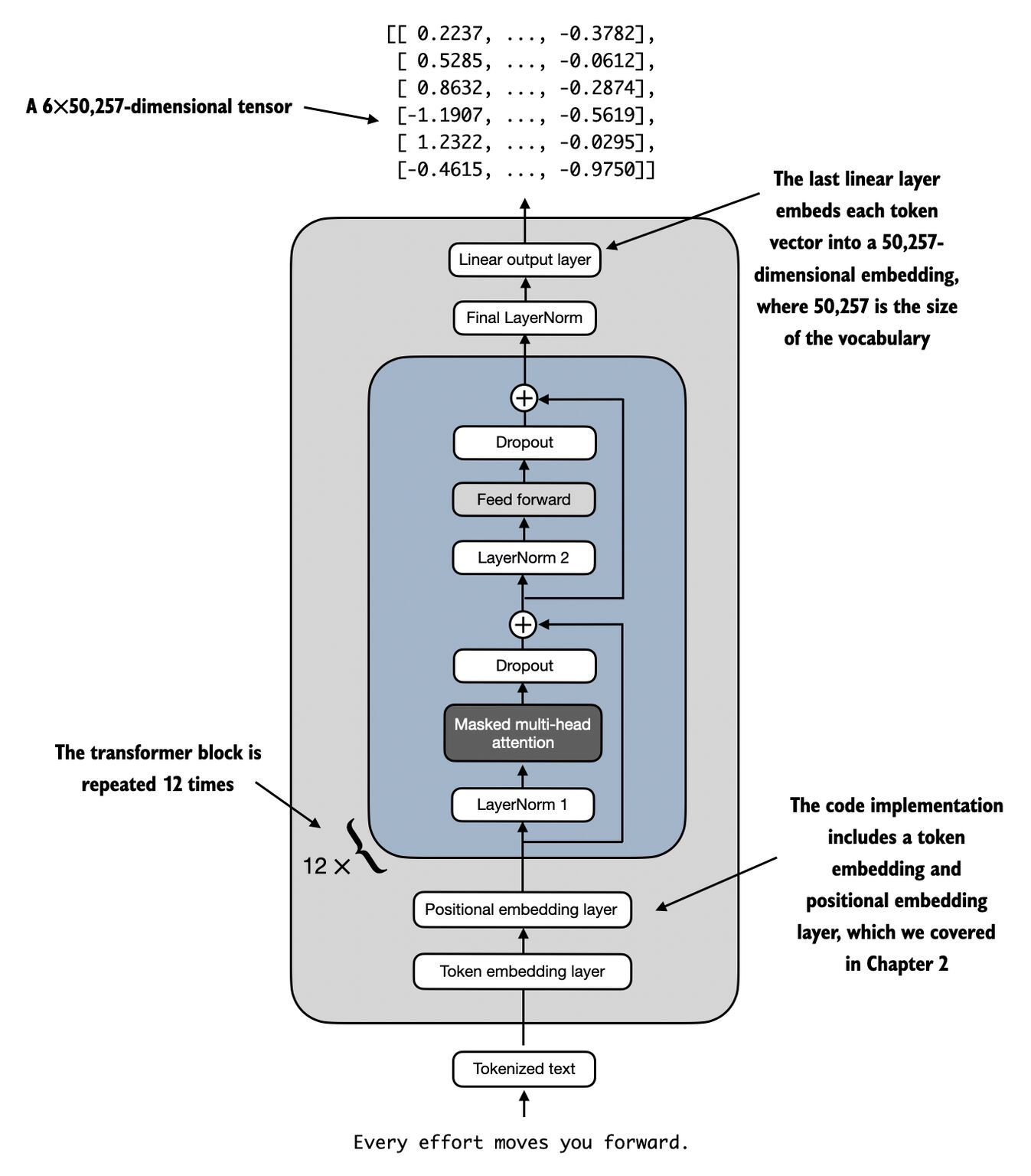
The GPT-2 architecture is a transformer-based model, and as the name
suggests, it is a continuation of the GPT-1 model with some minor modifications.
GPT-2 utilizes a Transformer architecture [Vaswani et al., 2017] as
its backbone, which is distinguished by self-attention mechanisms. In
short, we switched from bi-directional cross attention to uni-directional
self-attention.
Fig. 2 GPT Architecture. Image Credit: Build a Large Language Model (From Scratch) by Sebastian Raschka#
Layer normalization is repositioned to the input of each
sub-block, mirroring a pre-activation residual network. This
modification is believed to offer training stability and model performance.
By normalizing the inputs to each sub-block, it is conjectured to alleviate
issues tied to internal covariate shift, thus aiding in smoother and
potentially faster training.
GPT-2 introduces an additional layer normalization step that is
executed after the final self-attention block within the model. This
additional normalization step can help ensure that the outputs of the
transformer layers are normalized before being passed to subsequent layers
or used in further processing, further contributing to model stability.
The GPT-2 paper introduces a modification to the standard weight
initialization for the model’s residual layers. Specifically, the weights
are scaled by a factor of \(\frac{1}{\sqrt{N_{\text{decoder_blocks}}}}\),
where \(N_{\text{decoder_blocks}}\) represents the number of blocks (or
layers) in the Transformer’s decoder.
The rationale, as quoted from the paper: “A modified initialization which
accounts for the accumulation on the residual path with model depth is
used”[Radford et al., 2019], is to ensure that the variance of the
input to the block is the same as the variance of the block’s output. This
is to ensure that the signal is neither amplified nor diminished as it
passes through the block. As the model depth increases, the activations get
added/acculumated, and hence the scaling factor is
\(\frac{1}{\sqrt{N_{\text{decoder_blocks}}}}\), to scale it down.
Clearly, we can see the empahsis on model stability. In training large
language models, numerical stability is paramount; the cost of training
is significantly high, with every loss and gradient spike that fails to
recover necessitating a return to a previous checkpoint, resulting in
substantial GPU hours and potentially tens of thousands of dollars wasted.
The model’s vocabulary is expanded to 50,257 tokens.
The context window size is increased from 512 to 1024 tokens, enhancing the
model’s ability to maintain coherence over longer text spans.
A larger batch size of 512, GPT-2 benefits from more stable and effective
gradient estimates during training, contributing to improved learning
outcomes.
The GPT-2 paper introduces a modification to the standard weight
initialization for the model’s residual layers. Specifically, the weights
are scaled by a factor of \(\frac{1}{\sqrt{N_{\text{decoder_blocks}}}}\),
where \(N_{\text{decoder_blocks}}\) represents the number of blocks (or
layers) in the Transformer’s decoder.
The rationale, as quoted from the paper: “A modified initialization which
accounts for the accumulation on the residual path with model depth is
used”[Radford et al., 2019], is to ensure that the variance of the
input to the block is the same as the variance of the block’s output. This
is to ensure that the signal is neither amplified nor diminished as it
passes through the block. As the model depth increases, the activations get
added/acculumated, and hence the scaling factor is
\(\frac{1}{\sqrt{N_{\text{decoder_blocks}}}}\), to scale it down.
In practice, seeing how Karpathy implemented it, it seems that the
scalings are implemented on the projection layers of the
MultiHeadAttention and PositionwiseFFN layers, as seen below:
# apply special scaled init to the residual projections, per GPT-2 paperforpn,pinself.named_parameters():ifpn.endswith('c_proj.weight'):torch.nn.init.normal_(p,mean=0.0,std=0.02/math.sqrt(2*config.n_layer))
My guess is that the projection layers in both MultiHeadAttention and
PositionwiseFFN are critical junctures where the model’s representations
are linearly transformed. These layers significantly influence the
model’s ability to learn and propagate signals effectively through its
depth. Scaling the weights of these projection layers helps to control
the rate at which information (and error gradients) is dispersed
throughout the network, directly affecting learning stability and
efficiency.
I did not implement the custom scaling and just went ahead with default
weight scaling:
Weights initialization for the context projection and the context fully
connected layers are done using Xavier Uniform initialization.
def_init_weights(self)->None:"""Initialize parameters of the linear layers."""nn.init.xavier_uniform_(self.ffn["context_fc"].weight)ifself.ffn["context_fc"].biasisnotNone:nn.init.constant_(self.ffn["context_fc"].bias,0)nn.init.xavier_uniform_(self.ffn["context_projection"].weight)ifself.ffn["context_projection"].biasisnotNone:nn.init.constant_(self.ffn["context_projection"].bias,0)
To this end, we encapsulate some key parameters in
Table 4 below, which provides
specifications for several GPT-2 variants, distinguished by their scale.
Notice that the config does not show the dimension of the feedforward network.
In GPT-2 source code, we can see what the dimension of the feedforward network
is. It is defined as:
The shape is \(1 \times 8\), which is a single sequence of \(8\) tokens. And in this
case, we have each word/punctuation mapped to a unique token ID, as seen below.
Next, we need to map each token to a vector (embeddings) in a high-dimensional
space.
The integer tokens, by themselves, do not carry much information. For example,
the word priest is tokenized to be 11503, which is an arbitrary integer. In
a one-dimensional Euclidean space, the word priest and the next word and,
indexed by 290, would appear to be very far apart from each other.
However, if we were to change a tokenizer, and somehow the word priest is now
tokenized to be 291, then the words priest and andwould appear to be
very near to each other.
This means that the model could potentially learn the relationship of two tokens
based solely on their tokenized integers. To address this, we use embedding
vectors. While the initial mapping from words to vectors is dependent on the
tokenizer and may be arbitrary, during training, the model adjusts these
vectors so that words used in similar contexts come to have similar vectors.
This allows the model to capture semantic relationships between words - and
by extension, allows the model to capture relationships between tokens better.
Notice that for each token, the embedding vector is a \(4\)-dimensional vector.
This is because we have set the embedding dimension to be \(4\), which is a
hyperparameter that we can set. In the case of GPT-2, the embedding dimension is
\(768\).
Typically, the token embeddings are learned during training, and the learned
embeddings are used to represent the tokens in the input sequence.
We first unsqueeze the input tensor x0 to add a batch dimension, resulting
in a shape of [1,8] where 1 is the batch size \(\mathcal{B}\) and 8 is
the sequence length \(T\).
The tok_embed layer is then applied to the input tensor, resulting in a
tensor of shape [1,8,4].
z0_tok_embed is the token embedding tensor, which is the transformed
input tensor x0. Here our x0 was transformed from a sequence of
tokens to a sequence of token embeddings.
There is a weight matrix W_e that is [V,D] that transforms the input
tensor into the token embedding tensor via a matrix multiplication
z0_tok_embed=x0_ohe@W_e (which we will see shortly).
So this operation above is essentially a lookup operation, where we look up the
embedding vector for each token in the sequence. This is done by tok_embed(x).
We run it against the first sequence for simplicity, and z0_tok_embed is the
resulting tensor, with a shape of \(T \times D\). In our case, the sequence length
(block size) is \(T = 8\), and the embedding dimension is \(D = 4\). This means that
we have essentially mapped each of the \(8\) tokens representing
priestandclerk?wellthen,amen to a \(4\)-dimensional vector.
priest is mapped to [-1.0213,0.3146,-0.2616,0.3730]
and is mapped to [0.5715,0.1229,-0.8145,-1.4164]
…
amen is mapped to [1.2707,-0.5865,-1.4099,-1.3797]
With each token being a vector, not only does the token carry more information,
it is also much easier to do linear algebra operations on the tokens. For
example, we can easily calculate the mean/sum of the embeddings for pooling, or
we can easily calculate the dot product between two tokens to measure their
similarity in a high-dimensional space (as compared to it being an integer with
only 1 dimension).
Furthermore, the embeddings are learned during training, and the model would try
to capture semantic relationships between tokens. For example, the model would
try to learn that priest and clerk are related in some way because they
refer to people, and amen is related to priest because it is often used in
religious contexts.
To this end, we denote the output of the token embedding layer as \(\mathbf{X}\).
In what follows, we will see beneath how the token embedding layer is computed.
First, we need to understand how the input sequence \(\mathbf{x}\) can be
represented as a one-hot encoded matrix.
The one-hot representation of the input sequence \(\mathbf{x}\) is denoted as
\(\mathbf{X}^{\text{ohe}}\). This representation converts each token in the
sequence to a one-hot encoded vector, where each vector has a length equal to
the size of the vocabulary \(V\).
For each token \(x_t\) at position \(t\) in the sequence \(\mathbf{x}\)
(\(1 \leq t \leq T\)), the corresponding row vector \(\mathbf{o}_{t, :}\) in
\(\mathbf{X}^{\text{ohe}}\) is defined as:
Here, \(f_{\text{stoi}}(x_t)\) maps the token \(x_t\) to its index \(j-1\) in the
vocabulary \(\mathcal{V}\), the \(j-1\) is because zero-based indexing used in
python (where \(0 \leq j-1 < V\)). Each row \(\mathbf{o}_{t, :}\) in
\(\mathbf{X}^{\text{ohe}}\) contains a single ‘1’ at the column \(j\) corresponding
to the vocabulary index of \(x_t\), and ‘0’s elsewhere.
Example 2 (Example)
For example, if the vocabulary
\(\mathcal{V} = \{\text{cat}, \text{dog}, \text{mouse}\}\) and the sequence
\(\mathbf{x} = (\text{mouse}, \text{dog})\), then the one-hot encoded matrix
\(\mathbf{X}^{\text{ohe}}\) will be:
“mouse” corresponds to the third position in the vocabulary, and “dog” to
the second, which is seen in their respective one-hot vectors.
We write the one hot encoding proces for the input sequence x0 as follows
in python.
x0_ohe:torch.Tensor=F.one_hot(x0,num_classes=composer.vocab_size).float()assertx0_ohe.shape==(1,composer.block_size,composer.vocab_size)# [B, T, V] = [1, 8, 50257]forindex,token_idinenumerate(x0.squeeze()):assertx0_ohe[0,index,token_id].item()==1.0# check if the one-hot encoding is correct
Once the one hot encoding representation \(\mathbf{X}^{\text{ohe}}\) is well
defined, we can then pass it as input through our GPT model, in which the first
layer is a embedding lookup table. In the GPT model architecture, the first
layer typically involves mapping the one-hot encoded input vectors into a
lower-dimensional, dense embedding space using the embedding matrix
\(\mathbf{W}_e\).
Matrix Description
Symbol
Dimensions
Description
One-Hot Encoded Input Matrix
\(\mathbf{X}^{\text{ohe}}\)
\(T \times V\)
Each row corresponds to a one-hot encoded vector representing a token in the sequence.
Embedding Matrix
\(\mathbf{W}_e\)
\(V \times D\)
Each row is the embedding vector of the corresponding token in the vocabulary.
Embedded Input Matrix
\(\mathbf{X}\)
\(T \times D\)
Each row is the embedding vector of the corresponding token in the input sequence.
Embedding Vector for Token \(t\)
\(\mathbf{X}_t\)
\(1 \times D\)
The embedding vector for the token at position \(t\) in the input sequence.
Batched Input Tensor
\(\mathbf{X}^{\mathcal{B}}\)
\(B \times T \times D\)
A batched tensor containing \(B\) input sequences, each sequence is of shape \(T \times D\).
More concretely, we create an embedding matrix \(\mathbf{W}_{e}\) of size
\(V \times D\), where \(V\) is the vocabulary size, \(D\) is the dimensions of the
embeddings, we would then matrix multiply \(\mathbf{X}^{\text{ohe}}\) with
\(\mathbf{W}_{e}\) to get the output tensor \(\mathbf{X}\).
Indeed, we see that the result of tok_embed(x) is the same as the result of
x0_ohe@W_e. In other words, you can one hot encoded the input
sequence \(\mathbf{x} = (x_1, x_2, \ldots, x_T)\) and then matrix multiply it with
the embedding matrix \(\mathbf{W}^{e}\) (via a linear layer) to get the same
result as tok_embed(x).
W_e=tok_embed.embedding.weight.data# [V, D]x0_ohe:torch.Tensor=F.one_hot(x0,num_classes=composer.vocab_size).float()# [B, T, V]z0_tok_embed_matmul:torch.Tensor=x0_ohe@W_e# [B, T, D]assertz0_tok_embed_matmul.shape==(1,composer.block_size,composer.d_model)torch.testing.assert_close(z0_tok_embed,z0_tok_embed_matmul,rtol=0.0,atol=0.0,msg="The matrix multiplication is not correct.")
Recall our tokenized sequence is
[11503,290,21120,30,880,788,11,29448].
Converting it to one-hot encoding, we would have a matrix of size
[8,50257] (or more generally [B,T,V] in the presence of batch size
B).
Each row is a one-hot vector of the token \(x_{t} \in \mathbb{R}^{V}\) at
position \(t\). For example, the first row would be a one-hot vector of the
token 11503, so every element in the first row is \(0\) except for the
\(11503\)-th element, which is \(1\).
A minute quirk here is that the token \(x_{t}\) exists in the continuous
space instead of the discrete space. This is because we have to
perform the dot product between the one-hot vector and the embedding vector,
which is a continuous vector. This is more of a data type coercion.
Therefore, in our code, we also converted the one-hot vector to .float().
Each row vector \(\mathbf{w}_j\) of the matrix \(\mathbf{W}_e\) represents
the \(D\)-dimensional embedding vector for the \(j\)-th token in the
vocabulary \(\mathcal{V}\).
The subscript \(j\) ranges from 1 to \(V\), indexing the tokens.
\(V\) is the vocabulary size.
\(D\) is the hidden embedding dimension.
Here is a visual representation of how each embedding vector is selected through
matrix multiplication:
Each row in the resulting matrix \(\mathbf{X}\) is the embedding of the
corresponding token in the input sequence, picked directly from \(\mathbf{W}_e\)
by the one-hot vectors. In other words, the matrix \(\mathbf{W}_e\) can be
visualized as a table where each row corresponds to a token’s embedding vector:
When the one-hot encoded input matrix \(\mathbf{X}^{\text{ohe}}\) multiplies with
the embedding matrix \(\mathbf{W}_e\), each row of \(\mathbf{X}^{\text{ohe}}\)
effectively selects a corresponding row from \(\mathbf{W}_e\). This operation
simplifies to row selection because each row of \(\mathbf{X}^{\text{ohe}}\)
contains exactly one ‘1’ and the rest are ‘0’s.
Now each row of the output tensor, indexed by \(t\), \(\mathbf{X}_{t, :}\): is the
\(D\) dimensional embedding vector for the token \(x_t\) at the \(t\)-th position in
the sequence. In this context, each token in the sequence is represented by a
\(D\) dimensional vector. So, the output tensor \(\mathbf{X}\) captures the dense
representation of the sequence. Each token in the sequence is replaced by its
corresponding embedding vector from the embedding matrix \(\mathbf{W}_{e}\). As
before, the output tensor \(\mathbf{X}\) carries semantic information about the
tokens in the sequence. The closer two vectors are in this embedding space, the
more semantically similar they are.
For the lack of a better phrase, we say that self-attention, the core function
of GPTs, is permutation invariant. While it is obvious that the input sequence
\(\mathbf{x}\) is ordered in the sense that \(x_1\) comes before \(x_2\), and \(x_2\)
comes before \(x_3\), and so on, this information gets lost in the self-attention
mechanism. This means that the model does not differentiate “the cat ate the
mouse” from “the mouse ate the cat” as long as the tokens are the same - and
this is not desirable.
The dominant approach for preserving information about the order of tokens is to
represent this to the model as an additional input associated with each token.
These inputs are called positional encodings, and they can either be learned or
fixed a priori[Zhang et al., 2023]. What this means is that we can either
construct a learnable parameter that is updated during training, or we can
construct a fixed parameter that is not updated during training. For the sake of
completeness, we will discuss briefly the scheme where the positional encodings
are fixed a priori based on sinusoidal functions - which is also the scheme
described in the paper “Attention is All You Need” [Vaswani et al., 2017].
The positional encoding function
\(\mathrm{PE}: \mathbb{N} \times \mathbb{N} \rightarrow \mathbb{R}\) computes the
position encoding for each position \(p := t \in \mathbb{N}\) and each dimension
\(d = 1, 2, \ldots, D \in \mathbb{N}\) in the input embedding space as follows [Lee, 2023]:
\[\begin{split}
\operatorname{PE}(p, d)= \begin{cases}\sin \left(\frac{p}{10000^{\frac{2 d}{D}}}\right) & \text { if } d \text { is even, } \\ \cos \left(\frac{p}{10000^{\frac{2 d-1}{D}}}\right) & \text { if } d \text { is odd. }\end{cases}
\end{split}\]
It is worth noting that \(10,000\) is an parameter that can be changed.
Now to relate the positional encoding formula back to the implementation, we
would resume where we left off in the previous section. For a given input matrix
(token embedding matrix output) \(\mathbf{X} \in \mathbb{R}^{T \times D}\), where
\(T\) is the sequence length and \(D\) is the embedding dimension (denoted as
\(d_{\text{model}}\) in typical Transformer literature), the positional encoding
\(\operatorname{PE}\) is applied to integrate sequence positional information into
the embeddings. As a shorthand, the resultant matrix \(\mathbf{X}'\) (sometimes
denoted as \(\mathbf{P}\)) after applying positional encoding elementwise can be
expressed as follows:
for \(i = 1, \ldots, T\) and \(j = 1, \ldots, D\).
We can update our original embeddings tensor \(\mathbf{X}\) (recall this is the
output of the token embeddings layer) to include positional information:
Note that \(\mathbf{X}'= \operatorname{PE}(\mathbf{X})\) is independent of
\(\mathbf{Z}\), and it’s computed based on the positional encoding formula used in
transformers, which uses sinusoidal functions of different frequencies.
fromabcimportABC,abstractmethodimporttorchfromtorchimportnnclassPositionalEncoding(ABC,nn.Module):def__init__(self,d_model:int,context_length:int,dropout:float=0.0)->None:super().__init__()self.d_model=d_modelself.context_length=context_lengthself.dropout=nn.Dropout(p=dropout,inplace=False)@abstractmethoddefforward(self,x:torch.Tensor)->torch.Tensor:...classSinusoid(PositionalEncoding):P:torch.Tensordef__init__(self,d_model:int,context_length:int,dropout:float=0.0)->None:super().__init__(d_model,context_length,dropout)P=self._init_positional_encoding()self.register_buffer("P",P,persistent=True)# with this no need requires_grad=Falsedef_init_positional_encoding(self)->torch.Tensor:"""Initialize the positional encoding tensor."""P=torch.zeros((1,self.context_length,self.d_model))position=self._get_position_vector()div_term=self._get_div_term_vector()P[:,:,0::2]=torch.sin(position/div_term)P[:,:,1::2]=torch.cos(position/div_term)returnPdef_get_position_vector(self)->torch.Tensor:"""Return a vector representing the position of each token in a sequence."""returntorch.arange(self.context_length,dtype=torch.float32).reshape(-1,1)def_get_div_term_vector(self)->torch.Tensor:"""Return a vector representing the divisor term for positional encoding."""returntorch.pow(10000,torch.arange(0,self.d_model,2,dtype=torch.float32)/self.d_model,)defforward(self,z:torch.Tensor)->torch.Tensor:z=self._add_positional_encoding(z)z=self.dropout(z)returnzdef_add_positional_encoding(self,z:torch.Tensor)->torch.Tensor:"""Add the positional encoding tensor to the input tensor."""returnz+self.P[:,:z.shape[1],:]
We now do a sum operation between the output of the token embeddings \(\mathbf{Z}\)
and the positional encodings \(\mathbf{P}\) to get the final input to the model.
generator=torch.Generator(device=composer.device)generator.manual_seed(25)pos_embed=Sinusoid(d_model=composer.d_model,context_length=composer.block_size,dropout=0.0)P=pos_embed.Pz0_tok_embed_with_pos_embed=pos_embed(z0_tok_embed)z0_tok_embed_add_pos_embed=z0_tok_embed+Ptorch.testing.assert_close(z0_tok_embed_with_pos_embed,z0_tok_embed_add_pos_embed,rtol=0.0,atol=0.0)# just to show that adding P to the z0 is the same as pos_embed(z0)
As we have seen earlier using manual calculations, the input sequence’s first token/position at \(t=1\)
has values of \([0, 1, 0, 1]\) for the positional encoding with \(D=4\). We simply add this positional
encoding to the token embeddings to get the final input embeddings. We can verify it visually below (or can add programmatically).
This method slices the precalculated positional encodings tensor self.P to
match the sequence length of X, adds it to X, and then applies dropout. The
result, which is the sum of the original embeddings and the positional
encodings, is returned. So there’s no need to add the positional encodings to
X outside of this class.
So when you call pos_embed(Z_tok_embed), it adds the positional encodings to
Z_tok_embed and applies dropout, then returns the result. You could store this
result in Z_tok_embed_with_pos_embed.
Z_tok_embed_with_pos_embed=pos_embed(Z_tok_embed)
Now, Z_tok_embed_with_pos_embed contains the original embeddings with the
positional encodings added and dropout applied.
In the context of our “hello bot” example, the original tensor Z_tok_embed
represented the word embeddings, where each token in the sequence (i.e., SOS,
hello, bot, EOS) was converted into a 2-dimensional vector capturing the
semantic meaning of each token. After adding positional encoding, the new tensor
represents both the semantic and positional information of each token in the
sequence.
The first row ([1.1103,-0.6898]) now encapsulates both the meaning of the
SOS token and the information that it’s the first token in the sequence.
The second row ([0.0756,-0.2103]) is now a representation of the word
hello that carries not just its semantics (e.g., being a greeting), but
also the information that it’s the second word in the sentence.
The third row ([2.2618,0.2702]) likewise carries both the semantics of
bot (likely related to AI or technology), and its position as the third
word in the sentence.
The last row ([-0.8478,-0.0320]) encapsulates the semantics of EOS
token, signifying end of a sentence, and the fact that it’s the last token
in the sentence.
The idea here is that in natural language, word order matters. The sentence
“hello bot” is not the same as “bot hello” (okay maybe it is the same in this
example, a better one is cat eat mouse isn’t the same as mouse eat cat).
So, in a language model, we want our representations to capture not just what
words mean, but also where they are in a sentence. Positional encoding is a
technique to achieve this goal.
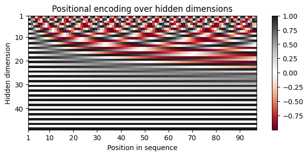
pos_embed_visual=Sinusoid(d_model=48,context_length=96)P_visual=pos_embed_visual.P.squeeze().T.cpu().numpy()fig,ax=plt.subplots(nrows=1,ncols=1,figsize=(8,3))pos=ax.imshow(P_visual,cmap="RdGy",extent=(1,P_visual.shape[1]+1,P_visual.shape[0]+1,1))fig.colorbar(pos,ax=ax)ax.set_xlabel("Position in sequence")ax.set_ylabel("Hidden dimension")ax.set_title("Positional encoding over hidden dimensions")ax.set_xticks([1]+[i*10foriinrange(1,1+P_visual.shape[1]//10)])ax.set_yticks([1]+[i*10foriinrange(1,1+P_visual.shape[0]//10)])plt.show()
The positional encodings are depicted through sine and cosine functions, each
varying in wavelength across the hidden dimensions, to uniquely represent each
position. By examining these functions within individual hidden dimensions, we
gain deeper insights into the encoding patterns. Here, we present a
visualization of the positional encodings across hidden dimensions \(d = 0, 1,
2, 3\) for the initial \(16\) sequence positions [Lippe, 2023].
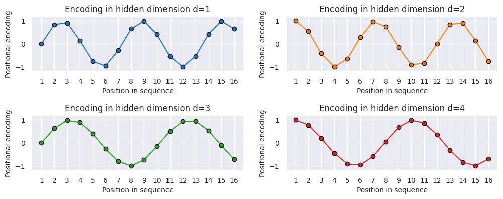
fromtypingimportList,Tupleimportnumpyasnpimportmatplotlib.pyplotaspltimportseabornassnsdefplot_positional_encoding(pe:np.ndarray,block_size:int,figsize:Tuple[int,int]=(12,4))->None:"""Plot positional encoding for each hidden dimension. Args: pe: Positional encoding array. composer_block_size: Block size of the composer. figsize: Figure size for the plot. """sns.set_theme()fig,ax=plt.subplots(2,2,figsize=figsize)ax=[afora_listinaxforaina_list]fori,ainenumerate(ax):a.plot(np.arange(1,block_size+1),pe[i,:block_size],color=f"C{i}",marker="o",markersize=6,markeredgecolor="black",)a.set_title(f"Encoding in hidden dimension d={i+1}")a.set_xlabel("Position in sequence",fontsize=10)a.set_ylabel("Positional encoding",fontsize=10)a.set_xticks(np.arange(1,17))a.tick_params(axis="both",which="major",labelsize=10)a.tick_params(axis="both",which="minor",labelsize=8)a.set_ylim(-1.2,1.2)fig.subplots_adjust(hspace=0.8)sns.reset_orig()plt.show()
plot_positional_encoding(P_visual,16)
As we can see, the patterns between the hidden dimension 1 and 2 only differ in
the starting angle. The wavelength is \(2\pi\) , hence the repetition after
position 6 . The hidden dimensions 2 and 3 have about twice the wavelength
[Lippe, 2023].
To demonstrate how positional encodings are calculated for an input sequence
using the given formula, let’s take the first three tokens from the example
sequence 'priestandclerk?wellthen,amen'. We’ll assume these tokens are
‘priest’, ‘and’, ‘clerk’ and that we’re dealing with an embedding dimension
\(D = 4\) for simplicity. The positions \(p\) of these tokens are 1, 2, and 3,
respectively.
For \(D = 4\), each token’s positional encoding will be a vector of 4 elements.
Let’s calculate the positional encodings for \(p = 1, 2, 3\) (corresponding to
‘priest’, ‘and’, ‘clerk?’) and for each dimension \(d = 0, 1, 2, 3\):
The uniqueness across different positions in the sequence is what’s important
For each token position (p): The encoding creates a vector of length D (4 in
the example).
Within each position’s vector: The values are calculated using alternating
sine and cosine functions across the dimensions (d=0 to d=3 in the example).
Across different positions: The key is that the encoding for position p=1 is
different from p=2, which is different from p=3, and so on.
The uniqueness comes from the combination of:
The position (p) changing for each token in the sequence
The dimension (d) varying within each token’s encoding
The use of different frequencies (controlled by 10000^(2d/D))
This creates a pattern where:
Each position has a unique overall encoding vector
Each dimension within that vector captures different aspects of the position
information
The relationship between encodings at different positions follows a
structured pattern
In practice, the positional encodings are learned as part of the GPT-2
[Radford et al., 2019]. So we can replicate the same by using a
nn.Embedding layer in PyTorch as in the token embeddings.
\(\mathbf{W}_{p}\) is the positional embedding matrix. Each row of this matrix
corresponds to the embedding of a position in a sequence. This matrix is usually
of size \(T \times D\), where \(T\) is the maximum length of a sequence we allow in
the model, and \(D\) is the dimension of the embedding space.
In other words, the \(\mathbf{P}\) positional matrix introduced earlier has the
same shape as \(\mathbf{W}_{p}\), and while the former is fixed, the latter is
learned during the training process.
To this end, we would have wrapped up the first two layers, where we first pass
an input sequence \(\mathbf{x}\) through the token embedding layer to obtain the
token embeddings \(\mathbf{X} = \mathbf{W}_{e} \mathbf{x}\), and then add the
positional embeddings to the token embeddings to obtain the final embeddings.
The process to encode position into the embeddings is:
Given an input sequence \(\mathbf{x} = \left(x_1, x_2, ..., x_{T}\right)\), where
\(x_t\) is the token at position \(t\) in the sequence, we have transformed the
input sequence into a sequence of token embeddings \(\mathbf{X}\), holding both
the static semantics and the positional information of the input sequence.
Layer normalization is a technique applied in the context of neural networks to
stabilize the learning process by normalizing the inputs across the features for
each token in a sequence. Given a data representation
\(\mathbf{Z} \in \mathbb{R}^{T \times D}\), where \(T\) is the sequence length
(number of tokens) and \(D\) is the hidden dimension (feature space), layer
normalization is applied independently to each vector (or token) across the
feature dimension \(D\). You can think of each token \(t=1, \ldots, T\) as a
separate example, and \(\mathbf{Z}_{t}\) represents each row/token. We then
compute the mean and variance for each row/token and then apply the
normalization to each row/token. This process is repeated for each row/token in
the input matrix \(\mathbf{Z}\).
When considering a batch of such sequences, represented as
\(\mathbf{Z}^{\mathcal{B}} \in \mathbb{R}^{\mathcal{B} \times T \times D}\), where
\(\mathcal{B}\) is the batch size, layer normalization still focuses on
normalizing each token vector within each sequence in the batch. The operation
does not aggregate or normalize across different tokens (\(T\) dimension) or
different sequences in the batch (\(\mathcal{B}\) dimension); instead, it
normalizes the values across the features (\(D\) dimension) for each token.
For a single token \(\mathbf{Z}_t \in \mathbb{R}^{1 \times D}\) in a sequence
\(\mathbf{Z} \in \mathbb{R}^{T \times D}\), the the normalization process involves
subtracting the mean \(\mu_t\) and dividing by the standard deviation \(\sigma_t\)
(adjusted with a small constant \(\epsilon\) for numerical stability) of its
features. This process ensures that, for each token, the features are centered
around zero with a unit variance.
Definition 4 (Layer Normalization)
Given a token \(\mathbf{Z}_t \in \mathbb{R}^{1 \times D}\) from the sequence
\(\mathbf{Z} \in \mathbb{R}^{T \times D}\), the normalized output
\(\overline{\mathbf{Z}}_t \in \mathbb{R}^{1 \times D}\) for this token can be
expressed as follows:
\(\mathbf{Z}_t\) is the vector of features for the token at position \(t\),
\(\mu_t \in \mathbb{R}\) is the mean of the features for this token,
\(\sigma_t^2 \in \mathbb{R}\) is the variance of the features for this token,
\(\epsilon \in \mathbb{R}\) is a small constant added for numerical stability,
ensuring that we never divide by zero or approach zero in the denominator.
The mean \(\mu_t\) and variance \(\sigma_t^2\) are computed as follows:
Here, \(\mathbf{Z}_{td}\) represents the \(d\)-th feature of the token at position
\(t\). The division and subtraction are applied element-wise across the feature
dimension \(D\) for the token, normalizing each feature based on the statistics of
the features within the same token.
Since layer normalization is performed for each token vector across the feature
dimension \(D\), the process can be vectorized and applied simultaneously to all
\(T\) token vectors in the sequence.
For each token \(t = 1, \ldots, T\), the mean \(\mu_t\) and variance
\(\sigma_t^2\) are computed.
Each token vector \(\mathbf{Z}_t\) is then normalized using its respective
\(\mu_t\) and \(\sigma_t^2\).
This results in a normalized sequence
\(\overline{\mathbf{Z}} \in \mathbb{R}^{T \times D}\), where each token vector
\(\overline{\mathbf{Z}}_t\) has been normalized independently. The normalized
sequence retains its original shape \((T \times D)\).
When considering a batch of sequences, represented as
\(\mathbf{Z}^{\mathcal{B}} \in \mathbb{R}^{\mathcal{B} \times T \times D}\), the
layer normalization process extends naturally:
The normalization process is applied independently to each token vector in
each sequence within the batch. This means for each sequence \(b\) in the
batch \(\mathcal{B}\), and for each token \(t\) in each sequence, the process
computes \(\mu_{bt}\) and \(\sigma_{bt}^2\), and normalizes each
\(\mathbf{Z}_{bt}\) accordingly.
Since the operation is independent across tokens and sequences, it can be
parallelized, allowing for efficient computation over the entire batch.
The result is a batch of normalized sequences,
\(\overline{\mathbf{Z}}^{\mathcal{B}} \in \mathbb{R}^{\mathcal{B} \times T \times D}\),
where each token vector \(\overline{\mathbf{Z}}_{bt}\) in each sequence of the
batch has been normalized based on its own mean and variance.
Broadcasting
It is worth noting that the notation above involves broadcasting, we are
essentially subtracting a scalar value (\(\mu_t\)) from a vector (\(\mathbf{Z}_t\))
and dividing by another scalar value (\(\sigma_t\)). This is fine in practice, as
the scalar values are broadcasted to match the shape of the vector during the
element-wise operations.
We can however make the definition clearer by removing the implicit
broadcasting, and say that for each activation \(Z_{td}\) (feature \(d\) of a token
at position \(t\)), we compute the normalized activation \(\overline{Z}_{td}\)
We see that indeed the assertion passed, and our calculations are correct. Note we must
set unbiased=False in the torch.var function to get the same result as the
LayerNorm function because we are using population variance formula.
We can further confirm below now the mean and variance close to 0 and 1 respectively.
mean=torch.mean(normalized_embedding,dim=-1)std=torch.std(normalized_embedding,dim=-1)print("\nExample of mean and std for a single sentence across embedding dimensions:")print("Mean:",mean[0])print("Standard deviation:",std[0])
Example of mean and std for a single sentence across embedding dimensions:
Mean: tensor([-3.7253e-08,  0.0000e+00, -5.9605e-08], grad_fn=<SelectBackward0>)
Standard deviation: tensor([1.1547, 1.1547, 1.1547], grad_fn=<SelectBackward0>)
Normalizing the activations to have zero mean and unit variance can limit the
representational power of the network, and thus after computing the normalized
features \(\hat{\mathbf{Z}}_t\) for each token, we introduce a learnable
affine transformation (scaling and shifting), in terms of parameters \(\gamma\)
and \(\beta\), which are of the same dimensionality as the feature space \(D\), to
scale and shift the normalized features, allowing the model to “undo” the
normalization if it is beneficial for the learning process.
where \(\overline{\mathbf{Z}}_t\) represents the output of the layer normalization
for the token at position \(t\), and \(\odot\) denotes element-wise multiplication.
And for each activation \(\mathbf{Z}_{td}\), we have:
where \(\gamma_d\) and \(\beta_d\) are the scaling and shifting parameters for the
\(d\)-th feature of the token at position \(t\). However notice that I did not
index \(\gamma\) and \(\beta\) by \(t\) because they are shared across all tokens in
the sequence.
The notation \(\gamma_{d}\) without indexing \(t\) implies that the scaling
parameter \(\gamma\) is feature-specific but shared across all tokens in the
sequence. It means that each feature dimension \(d\) across all tokens \(t\) in the
sequence has its own unique scaling parameter, but this parameter does not
change with different tokens. This is the common setup in layer normalization,
where \(\gamma\) and \(\beta\) parameters are learned for each feature dimension \(D\)
and are applied identically across all tokens \(T\).
Overall, layer norm is just taking each row in \(\mathbf{Z}\), sum all \(D\)
elements in the row, and then calculate the mean and variance. Then, we subtract
the mean from each element in the row, divide by the standard deviation, and
then scale and shift the result using \(\gamma\) and \(\beta\).
Besides the known fact that layer normalization enables convergence and provdies
regularization [Lippe, 2023], it also stabilizes the distributions of
activations [Zhang et al., 2023]. Training deep neural networks are
challenging, loss can easily be exploded or vanished, and the gradients can be
unstable. One simple way is to ensure each layer’s activation has a similar
distribution - the intuition is that if each layer’s activation has a similar
distribution, then the gradients will also have a similar distribution, and this
will stabilize the training process. Layer normalization is one of the
techniques that can help to achieve this.
I have written a more detailed post on the intuition of
ResNet
which is heavily adapted from the chapter
Residual Networks (ResNet) and ResNeXt
from the Dive into Deep Learning book.
For the sake of intuition, we can think of the residual connection as a way to
ensure that the original input to a layer is not lost as it passes through the
model layers.
Deep neural networks are known to suffer from the vanishing gradient
problem, where gradients become increasingly small as they are
backpropagated through the layers during training. Since we are
backpropagating backwards, the earlier layers are therefore more susceptible
to this problem. The weak gradient signal could often be close to \(0\), and
this could lead to the model not learning well. Consequently, we mitigate
this problem by adding the original input to the output of the layer, so
that the gradient signal has a direct path to flow through the network.
Furthermore, Eugene Yan’s blog post
Some Intuition on Attention and the Transformer
also highlighted that attention acting as a filtering mechanism may
block information from passing through, directly resulting flat
gradients as a small change to the inputs of the attention layer may not
change the outputs that much. Skip (residual) connections help resolve
this.
We will see later that Multi-Head Attention mechanism operates on a set of
tokens, instead of over a sequence. We encode positional information into
the tokens, but there is a risk that the positional information is lost in
the multi-head attention layers. The residual connection helps to ensure
that the positional information is not lost [Lippe, 2023].
The other well known property of the residual connection is that it helps to
learn the identity function. Perhaps the scenario is that the best thing a
layer or a series of layer can learn is itself - and we don’t actually want
an update.
We quote the following from the Dive into Deep Learning book:
Consider \(\mathcal{F}\), the class of functions that a specific network
architecture (together with learning rates and other hyperparameter settings)
can reach. That is, for all \(f \in \mathcal{F}\) there exists some set of
parameters (e.g., weights and biases) that can be obtained through training on a
suitable dataset. Let us assume that \(f^*\) is th “truth” function that we really
would like to find. If it is in \(\mathcal{F}\), we are in good shape but
typically we will not b quite so lucky. Instead, we will try to find some
\(f_{\mathcal{F}}^*\) which is our best bet within \(\mathcal{F}\). For instance,
given a dataset with features \(\mathbf{X}\) and labels \(\mathbf{y}\), we might try
finding it by solving the following optimization problem:
\[
f_{\mathcal{F}}^* \stackrel{\text { def }}{=} \underset{f}{\operatorname{argmin}} L(\mathbf{X}, \mathbf{y}, f) \text { subject to } f \in \mathcal{F} .
\]
It is only reasonable to assume that if we design a different and more powerful
architecture \(\mathcal{F}^{\prime}\) we should arrive at a better outcome. In
other words, we would expect that \(f_{\mathcal{F}}^*\) is “better” than
\(f_{\mathcal{F}}^*\). However, if \(\mathcal{F} \nsubseteq \mathcal{F}^{\prime}\)
there is no guarantee that this should even happen. In fact,
\(f_{\mathcal{F}^{\prime}}^*\) might well be worse.
As illustrated by Fig. 3, for non-nested function
classes, a larger function class does not always move closer to the “truth”
function \(f^*\). For instance, on the left of
Fig. 3, though
\(\mathcal{F}_3\) is closer to \(f^*\) than \(\mathcal{F}_1, \mathcal{F}_6\) moves
away and there is no guarantee that further increasing the complexity can reduce
the distance from \(f^*\). With nested function classes where
\(\mathcal{F}_1 \subseteq \ldots \subseteq \mathcal{F}_6\) on the right of
Fig. 3, we can avoid the aforementioned issue from
the non-nested function classes.
Fig. 3 For non-nested function classes, a larger (indicated by area) function class
does not guarantee we will get closer to the “truth” function \(f^*\). This
does not happen for nested function classes.#
where the layernorm is applied after the residual connection. In other words, if
Sublayer is a function that represents a sublayer (e.g.,
MultiHeadAttention), then in each sub-block of the decoder, we would compute
the output and then add the original input to the output, and then apply layer
normalization to the sum.
However, in GPT-2, there is a modification, more concretely, to shift the layer
normalization to the input of the sub-block. This means now instead of applying
layer normalization after the residual connection, we apply it before the
residual connection. For example, if Sublayer is a function that represents a
sublayer (e.g., MultiHeadAttention), then in each sub-block of the decoder, we
would first apply layer normalization to the input, then pass the normalized
input to the sublayer, and then add the original input to the output of the
sublayer.
fromtypingimportCallableimporttorchfromtorchimportnnclassResidualBlock(nn.Module):defforward(self,x:torch.Tensor,sublayer:Callable[[torch.Tensor],torch.Tensor],)->torch.Tensor:returnx+sublayer(x)classAddNorm(nn.Module):def__init__(self,feature_dim:int,dropout:float)->None:super().__init__()# fmt: offself.dropout=nn.Dropout(p=dropout,inplace=False)self.layer_norm=LayerNorm(normalized_shape=feature_dim,eps=1e-5,elementwise_affine=True)# fmt: ondefforward(self,x:torch.Tensor,sublayer:Callable[[torch.Tensor],torch.Tensor])->torch.Tensor:"""G(F(x) + x) where G = layer norm and F = sublayer"""# FIXME: GPT-2 should be x + self.dropout(sublayer(self.layer_norm(x)))output:torch.Tensor=self.layer_norm(x+sublayer(self.dropout(x)))returnoutput
We may have used \(\mathbf{X}\) to represent the output of the token and positional
embedding layer, but in what follows we probably will default to using \(\mathbf{Z}\).
Attention is not a new concept, and one of the most influencial papers came from
Neural Machine Translation by Jointly Learning to Align and Translate[Bahdanau et al., 2014], a paper published during 2014. In the context of our
post, we would stick to one intuitive interpretation, that the attention
mechanism describes a weighted average of (sequence) elements with the
weights dynamically computed based on an input query and elements’ keys[Lippe, 2023]. In other words, we want contextually relevant
information to be weighted more heavily than less relevant information. For
example, the sentence the cat walks by the river bank would require the word
bank to be weighted more heavily than the word the when the word cat is
being processed. The dynamic portion is also important because this allows the
model to adjust the weights based on an input sequence (note that the learned
weights are static but the interaction with the input sequence is dynamic). When
attending to the token cat in the sequence, we would want the token
cat to be a weighted average of all the tokens in the sequence, including
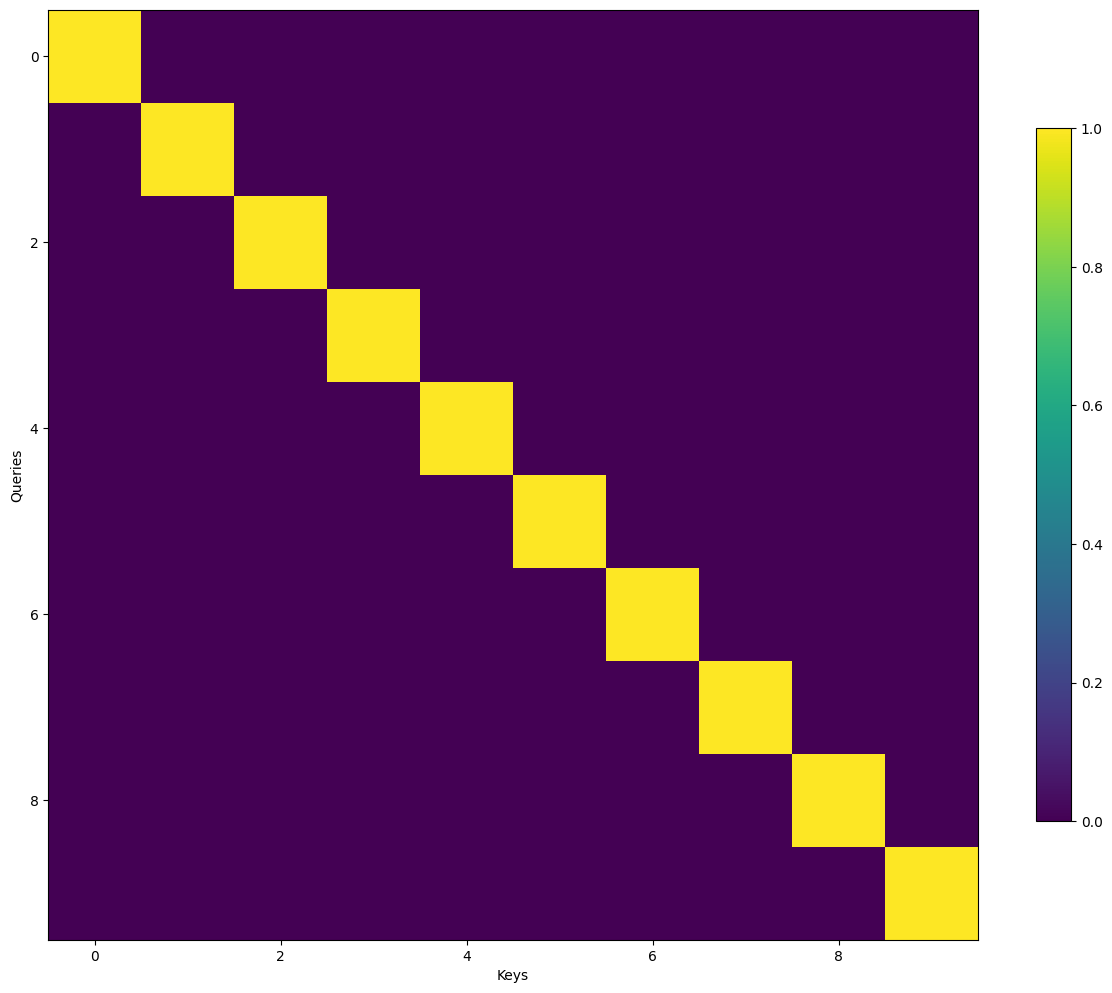
itself. This is the essence of the self-attention mechanism. Note carefully that
at this point we do not assume that the self-attention is causal as we want to
discuss it generally first.
Given an input sequence \(\mathbf{x} = \left(x_1, x_2, \ldots, x_T\right)\), where
\(T\) is the length of the sequence, and each \(x_t \in \mathcal{V}\) is a token in
the sequence, we use a generic embedding function \(h_{\text{emb}}\) to map each
token to a vector representation in a continuous vector space:
where \(\mathcal{V}\) is the vocabulary of tokens (discrete space \(\mathbb{Z}\)),
and \(D\) is the dimension of the embedding space (continuous space). The output
of the embedding function \(h_{\text{emb}}\) is a sequence of vectors
\(\mathbf{Z} = \left(\mathbf{z}_1, \mathbf{z}_2, \ldots, \mathbf{z}_T\right)\),
where each \(\mathbf{z}_t \in \mathbb{R}^{D}\) is the vector representation of the
token \(x_t\) in the sequence. As seen earlier, we represent the sequence of
vectors \(\mathbf{Z}\) as a matrix \(\mathbf{Z} \in \mathbb{R}^{T \times D}\), where
each row of the matrix represents the vector representation of each token in the
sequence.
Let’s draw an analogy to understand the concept of queries, keys, and values in
the context of the attention mechanism. Consider a database \(\mathcal{D}\)
consisting of tuples of keys and values. For instance, the database
\(\mathcal{D}\) might consist of tuples
{("Zhang","Aston"),("Lipton","Zachary"),("Li","Mu"),("Smola","Alex"),("Hu","Rachel"),("Werness","Brent")}
with the last name being the key and the first name being the value
[Zhang et al., 2023]. Operations on the database \(\mathcal{D}\) can be performed
using queries \(q\) that operate on the keys and values in the database. More
concretely, if our query is “Li”, or more verbosely, “What is the first name
associated with the last name Li?”, the answer would be “Mu” - the key
associated with the query “What is the first name associated with the last
name Li?” is “Li”, and the value associated with the key “Li” is “Mu”.
Furthermore, if we also allowed for approximate matches, we would retrieve
(“Lipton”, “Zachary”) instead.
More rigorously, we denote
\(\mathcal{D} \stackrel{\text { def }}{=}\left\{\left(\mathbf{k}_1, \mathbf{v}_1\right), \ldots\left(\mathbf{k}_m, \mathbf{v}_m\right)\right\}\)
a database of \(m\) tuples of keys and values, as well as a query
\(\mathbf{q}\). Then we can define the attention over \(\mathcal{D}\) as
where
\(\alpha\left(\mathbf{q}, \mathbf{k}_t\right) \in \mathbb{R}(t=1, \ldots, T)\) are
scalar attention weights [Zhang et al., 2023]. The operation itself is
typically referred to as
attention pooling.
The term “attention” is used because this operation focuses specifically on
those terms that have a substantial weight, denoted as \(\alpha\), meaning it
gives more importance to these terms. Consequently, the attention over
\(\mathcal{D}\) generates a linear combination of values contained in the
database. In fact, this contains the above example as a special case where all
but one weight is zero. Why so? Because the query is an exact match for one of
the keys.
To illustrate why in the case of an exact match within a database the attention
weights (\(\alpha\)) are all zero except for one, let’s use the attention formula
provided and consider a simplified example with vectors.
Example 3 (Exact Match Scenario)
Imagine a simplified database \(\mathcal{D}\) consisting of 3 key-value pairs,
where each key \(\mathbf{k}_t\) and the query \(\mathbf{q}\) are represented as
vectors in some high-dimensional space, and the values \(\mathbf{v}_t\) are also
vectors (or can be scalar for simplicity in this example). For simplicity, let’s
assume our vectors are in a 2-dimensional space and represent them as follows:
Keys (representing \(3\) keys in the database):
\(\mathbf{k}_1 = [1, 0]\),
\(\mathbf{k}_2 = [0, 1]\),
\(\mathbf{k}_3 = [1, 1]\)
Values (corresponding to the keys):
\(\mathbf{v}_1 = [0.1, 0.9]\),
\(\mathbf{v}_2 = [0.2, 0.8]\),
\(\mathbf{v}_3 = [0.3, 0.7]\)
Query (looking for an item/concept similar to \(\mathbf{k}_1\)):
\(\mathbf{q} = [1, 0]\)
The attention weights \(\alpha(\mathbf{q}, \mathbf{k}_t)\) indicate how similar or
relevant each key is to the query. In an exact match scenario, the similarity
calculation will result in a high value (e.g., \(1\)) when the query matches a key
exactly, and low values (e.g., \(0\)) otherwise. For simplicity, let’s use a
simple matching criterion where the weight is \(1\) for an exact match and \(0\)
otherwise:
This calculation shows that because the attention weights for \(\mathbf{k}_2\) and
\(\mathbf{k}_3\) are zero (due to no exact match), they don’t contribute to the
final attention output. Only \(\mathbf{k}_1\), which exactly matches the query,
has a non-zero weight (1), making it the sole contributor to the attention
result. This is a direct consequence of the query being an exact match for one
of the keys, leading to a scenario where “all but one weight is zero.”
The database example is a neat analogy to understand the concept of queries,
keys, and values in the context of the attention mechanism. To put things into
perspective, each token \(x_t\) in the input sequence \(\mathbf{x}\) emits three
vectors through projecting its corresponding token and positional embedding
output \(\mathbf{z}_t\), a query vector \(\mathbf{q}_t\), a key vector
\(\mathbf{k}_t\), and a value vector \(\mathbf{v}_t\). Consider the earlier example
cat walks by the river bank, where each word is a token in the sequence. When
we start to process the first token \(\mathbf{z}_1\), cat, we would consider a
query vector \(\mathbf{q}_1\), projected from \(\mathbf{z}_1\), to be used to
interact with the key vectors \(\mathbf{k}_t\) for \(t \in \{1, 2, \ldots, T\}\), in
the sequence - determining how much attention “cat” should pay to every other
token in the sequence (including itself). Consequently, it will also emit a key
vector \(\mathbf{k}_1\) so that other tokens can interact with it. Subsequently,
the attention pooling will form a linear combination of the query vector
\(\mathbf{q}_1\) with every other key vector \(\mathbf{k}_t\) in the sequence,
and each \(\alpha(\mathbf{q}_1, \mathbf{k}_t)\) will indicate how much attention
the token “cat” should pay to the token at position \(t\) in the sequence. We
would later see that we would add a softmax normalization to the attention
scores to obtain the final attention weights.
We would then use the attention scores \(\alpha(\mathbf{q}_1, \mathbf{k}_t)\) to
create a weighted sum of the value vectors \(\mathbf{v}_t\) to form the new
representation of the token “cat”.
Consequently, the first token must also emit a value vector \(\mathbf{v}_1\). You
can think of the value vector as carrying the actual information or content that
will be aggregated based on the attention scores.
To reiterate, the output
\(\operatorname{Attention}(\mathbf{q}_1, \mathbf{k}_t, \mathbf{v}_t)\) will be the
new representation of the token “cat” in the sequence, which is a weighted sum
of the value vectors \(\mathbf{v}_t\) based on the attention scores
\(\alpha(\mathbf{q}_1, \mathbf{k}_t)\) and now not only holds semantic and
positional information about the token “cat” itself but also contextual
information about the other tokens in the sequence. This allows the token “cat”
to have a better understanding of itself in the context of the whole sentence.
In this whole input sequence, the most ambiguous token is the token “bank” as it
can refer to a financial institution or a river bank. The attention mechanism
will help the token “bank” to understand its context in the sentence - likely
focusing more on the token “river” than the token “cat” or “walks” to understand
its context.
The same process will be repeated for each token in the sequence, where each
token will emit a query vector, a key vector, and a value vector. The attention
scores will be calculated for each token in the sequence, and the weighted sum
of the value vectors will be used to form the new representation of each token
in the sequence.
To end this off, we can intuitively think of the query, key and value as
follows:
Query: What does the token want to know? Maybe to the token bank, it
is trying to figure out if it is a financial institution or a river bank.
But obviously, when considering the token “bank” within such an input
sequence, the query vector generated for “bank” would not actually ask “Am I
a financial institution or a river bank?” but rather would be an abstract
feature vector in a \(D\) dimensional subspace that somehow captures the
potential and context meanings of the token “bank” and once it is used to
interact with the key vectors, it will help to determine later on how much
attention the token “bank” should pay to the other tokens in the sequence.
Key: Carrying on from the previous point, if the query vector for the
token “bank” is being matched with the key vectors of the other tokens in
the sequence, the key “river” will be a good match for the query “bank” as
it will help the token “bank” to understand its context in the sentence. In
this subspace, the key vector for “river” will be a good match for the query
because it is more of an “offering” service to the query vector, and it will
know when it is deemed to be important to the query vector. As such, the
vectors in this subspace are able to identify itself as important or not
based on the query vector.
Value: The value vector is the actual information or content that will
be aggregated based on the attention scores. If the attention mechanism
determines that “river” is highly relevant to understanding the context of
“bank” within the sentence, the value vector associated with “river” will be
given more weight in the aggregation process. This means that the
characteristics or features encoded in the “river” value vector
significantly influence the representation of the sentence or the specific
context being analyzed.
We have discussed the concept of queries, keys, and values but have not yet
discussed how these vectors are obtained. As we have continuously emphasized,
the query, key, and value vectors lie in a \(D\)-dimensional subspace, and they
encode various abstract information about the tokens in the sequence.
Consequently, it is no surprise that these vectors are obtained through linear
transformations/projections of the token embeddings \(\mathbf{Z}\) using learned
weight matrices \(\mathbf{W}^{\mathbf{Q}}\), \(\mathbf{W}^{\mathbf{K}}\) and
\(\mathbf{W}^{\mathbf{V}}\).
Definition 5 (Linear Projections for Queries, Keys, and Values)
In the self-attention mechanism, each token embedding
\(\mathbf{z}_t \in \mathbb{R}^{D}\) is projected into a new context vector across
different subspaces. This projection is accomplished through three distinct
linear transformations, each defined by a unique weight matrix:
where \(d_q, d_k, d_v \in \mathbb{Z}^+\) are the hidden dimensions of the
subspaces for the query, key, and value vectors, respectively.
Remark 3 (Dimensionality of the Subspaces)
It is worth noting that this post is written in the context of understand
GPT models, and the dimensionality of the query, key, and value vectors are
the same and usually equal to the dimensionality of the token embeddings.
Thus, we may use \(D\) interchangeably to indicate \(d_k, d_v\) and \(d_q\). This
is not always the case, as encoder-decoder models might have different
dimensionalities for the query, key, and value vectors. However, query and key
must have the same dimensionality for the dot product to work.
Each token embedding \(\mathbf{z}_t\) is transformed into three vectors:
The query vector\(\mathbf{q}_t\), representing what the token is looking
for in other parts of the input,
The key vector\(\mathbf{k}_t\), representing how other tokens can be
found or matched,
The value vector\(\mathbf{v}_t\), containing the actual information to be
used in the output.
where each row of these matrices corresponds to the query, key, and value
vectors for each token, respectively.
These matrices are generated through simple matrix multiplication of the token
embedding matrix \(\mathbf{Z} \in \mathbb{R}^{T \times D}\) with the weight
matrices
\(\mathbf{W}^{\mathbf{Q}}, \mathbf{W}^{\mathbf{K}}\) and \(\mathbf{W}^{\mathbf{V}}\):
The attention mechanism is a function that maps a set of queries, keys, and
values to an output, all of which are represented as matrices in a
\(D\)-dimensional space. Specifically, the function is defined as:
where given a query matrix \(\mathbf{Q} \in \mathbb{R}^{T \times d_q}\), a key
matrix \(\mathbf{K} \in \mathbb{R}^{T \times d_k}\), and a value matrix
\(\mathbf{V} \in \mathbb{R}^{T \times d_v}\), the attention mechanism computes the
the output matrix as follows:
\(\mathbf{Q}\mathbf{K}^{\top}\) represents the dot product between the query
and key matrices, resulting in a matrix of scores that indicate the degree
of alignment or relevance between each query and all keys.
\(\sqrt{d_k}\) is a scaling factor used to normalize the scores, preventing them
from becoming too large and ensuring a stable gradient during training. This
scaling factor is particularly important as it helps maintain the softmax
output in a numerically stable range [Vaswani et al., 2017].
\(\text{softmax}(\cdot)\) is applied row-wise to convert scores into attention
weights, ensuring that for each query, the weights across all keys sum up
to 1. This normalization step allows the mechanism to effectively distribute
focus across the keys according to their relevance to each query.
The resulting matrix of attention weights is then used to compute a weighted
sum of the values in \(\mathbf{V}\), producing the output matrix. This output
represents a series of context vectors, each corresponding to a query and
containing aggregated information from the most relevant parts of the input
sequence as determined by the attention weights.
In what follows, we will break down the components of the attention mechanism
and explain how it works in detail:
In order to know which tokens in the sequence are most relevant to the current
token, we need to calculate the attention scores between the query and key
vectors. Consequently, we would need a scoring function that measures the
influence or contribution of the \(j\)-th position on the \(i\)-th position in the
sequence. This is achieved through the dot product between the query and key
vectors, the reasoning through a
Gaussian kernel is rigorous and
provides a good
intuition
why we chose the dot product as the scoring function (other than the fact that
it is a measure of similarity).
Definition 7 (Attention Scoring Function)
Define the attention scoring function \(\alpha(\cdot)\) as a function
that calculates the relevance or influence of each position \(t\) in the sequence
on position \(i\), known as the attention scores. The attention scoring function
\(\alpha(\cdot)\) is defined using the dot product between query and key
vectors, leveraging its property as a similarity measure.
\(\mathbf{q}\) is a query vector representing in the sequence, seeking
information or context.
\(\mathbf{k}_t\) is the key vector representing the \(t\)-th position in the
sequence, offering context or information.
\(\langle \mathbf{q}, \mathbf{k}_t \rangle\) denotes the dot product between
the query vector \(\mathbf{q}\) and the key vector \(\mathbf{k}_t\), which
quantifies the level of similarity or alignment between the current position
that \(\mathbf{q}\) is at (say \(i\)-th) and \(t\)-th positions in the sequence.
The expression \(\mathbf{q} \cdot \mathbf{k}_t\) is a scalar value that indicates
the degree of alignment or relevance between the query at \(i\)-th position and
the key at \(t\)-th position in the sequence. We would need to calculate the
attention scores for each token in the sequence with respect to the query vector
\(\mathbf{q}\), and the key vectors \(\mathbf{k}_t\) for
\(t \in \{1, 2, \ldots, T\}\).
is the matrix of key vectors for each token in the sequence, and the output
\(\alpha(\mathbf{q}, \mathbf{K}) \in \mathbb{R}^{1 \times T}\) is a row
vector of attention scores for the query vector \(\mathbf{q}\) with respect to
each key vector \(\mathbf{k}_t\) for \(t \in \{1, 2, \ldots, T\}\).
Lastly, there are \(T\) such queries in the input sequence \(\mathbf{Q}\), and we
can stack all the query vectors \(\mathbf{q}_t\) into a matrix
\(\mathbf{Q} \in \mathbb{R}^{T \times d_q}\) to calculate the attention scores for
all the queries in the sequence with respect to all the key vectors in the
sequence.
To this end, each row of the matrix \(\mathbf{Q}\mathbf{K}^{\top}\) represents the
attention scores for each query vector at position \(i\) in the sequence with
respect to all the key vectors in the sequence.
Definition 8 (Query and Key are Independent and Identically Distributed (i.i.d.))
Under the assumption of the query \(\mathbf{q}\) and key \(\mathbf{k}_t\) are
independent and identically distributed (i.i.d.) random variables with a
gaussian distribution of mean \(0\) and variance \(\sigma^2\):
Given that \(\mathbf{q} \overset{\mathrm{iid}}{\sim} \mathcal{N}(0, \sigma^2), \quad \mathbf{k}_t \overset{\mathrm{iid}}{\sim} \mathcal{N}(0, \sigma^2)\),
the variance of the dot product between the query vector \(\mathbf{q}\) and the key
vector \(\mathbf{k}_t\) is:
where \(q_i\) and \(k_{ti}\) are the \(i\)-th components of \(\mathbf{q}\) and
\(\mathbf{k}_t\), respectively.
The variance of the sum of random variables (when these variables are
independent, which is our case since components are iid) is the sum of their
variances. The product \(q_i k_{ti}\) is a new random variable, and its variance
can be calculated as follows for a single pair of components:
Since \(\mathbb{E}[q_i k_{ti}] = 0\), the variance of the product \(q_i k_{ti}\) is
simply \(\sigma^4\).
For the dot product, we sum across all \(d_k\) components, and since the variance
of the sum of independent random variables is the sum of their variances:
We want to ensure that the variance of the dot product still remains the same as
the variance of the query and key vectors at \(\sigma^2\) regardless of the vector
dimensions. To do so, we scale down the dot product by \(\sqrt{d_k}\), which is
the square root of the dimensionality of the key vectors, this operation would
scale the variance of the dot product down by \(\sqrt{d_k}^2 = d_k\) (since
variance of a scaled random variable is the square of the scale factor times the
original variance).
Now our variance would be \(\sigma^4\) - but it is still not the same as the
variance of the query and key vectors. This is okay because the original paper
assume the variance \(\sigma^2 = 1\)[Vaswani et al., 2017], and therefore
it does not matter since \(\sigma^2 = \sigma^4\) when \(\sigma^2 = 1\).
Definition 10 (Attention Scoring Function with Scaling)
Before we look into the reason why we scale down the dot product, let’s first
complete the final block of the attention mechanism, which is the softmax
normalization.
Currently the attention scores \(\alpha(\mathbf{Q}, \mathbf{K})\) are raw scores
that indicate the degree of alignment or relevance between each query and all
keys. They can be negative or positive, and they can be large or small. We
denote them as the raw attention scores\(\alpha(\mathbf{Q}, \mathbf{K}) \in
\mathbb{R}^{T \times T}\).
Definition 12 (Softmax Normalization and Attention Weights)
It is common in deep learning to form a convex combination [Zhang et al., 2023]
of the attention scores \(\alpha(\mathbf{Q}, \mathbf{K})\) to obtain the
attention weights, denoted as \(\text{softmax}(\alpha(\mathbf{Q}, \mathbf{K}))\), which
are non-negative and sum to \(1\). This is achieved through the softmax
normalization function, which is defined as:
\(\exp(\cdot)\) is the exponential function, which is applied element-wise to
the raw attention scores \(\alpha(\mathbf{Q}, \mathbf{K})\).
The denominator is the sum of the exponentials of the raw attention scores
across the \(T\) keys, ensuring that the attention weights sum to \(1\) for
each query, allowing the mechanism to effectively distribute focus across
the keys according to their relevance to each query.
The choice of softmax is a convenient choice, but not the only choice. However,
it is convenient because it is both differentiable, which is often a desirable
property for training deep learning models that are optimized using
gradient-based methods, and it is also monotonic, which means that the
attention weights are preserved exactly in the order as the raw attention
scores.
Definition 13 (Attention Scoring Function with Scaling and Softmax)
To this end, our final attention scoring function is:
Consequently, we complete the walkthrough of the scaled dot-product attention
mechanism by calculating the context vector, which is the weighted sum of the
value vectors based on the attention weights obtained from the softmax
normalization.
Definition 14 (Context Vector/Matrix)
Given the attention weights \(\alpha(\mathbf{Q}, \mathbf{K})\) and the value
matrix \(\mathbf{V}\), the context vector \(\mathbf{C}\) is defined as the output
of the scaled dot-product attention mechanism:
where each row \(\mathbf{c}_t\) of the context matrix \(\mathbf{C}\) is the
new embedding of the token at position \(t\) in the sequence, containing
not only the semantic and positional information of the token itself, but also
contextual information from the other tokens in the sequence.
We can now revisit on the underlying reason why we scale down the dot product
\(\mathbf{Q}\mathbf{K}^{\top}\) by \(\sqrt{d_k}\).
First, the softmax function has all the desirable properties we want,
smoothness, monotonicity, and differentiability, but it is sensitive to
large input values.
The softmax function is defined as follows for a given logit \(z_i\) among a set
of logits \(Z\):
If the variance of the logits before applying softmax is too large (not scaled
down to a more manageable range), the exponential function \(e^{z_i}\) can lead to
extremely large output values for any \(z_i\) that is even slightly larger than
others in the set. This is due to the exponential function’s rapid growth with
respect to its input value.
Remark 4 (Gradient Saturation)
For one random element: If one of the logits \(z_i\) is significantly
larger than the others (which is more likely when the variance of the logits
is high), \(e^{z_i}\) will dominate the numerator and denominator of the
softmax function for this logit. This will cause the softmax output for this
logit to approach 1, as it essentially overshadows all other \(e^{z_j}\) terms
in the denominator.
For all others: Simultaneously, the softmax outputs for all other logits
\(z_j\) (where \(j \neq i\)) will approach 0, because their \(e^{z_j}\)
contributions to the numerator will be negligible compared to \(e^{z_i}\) in
the denominator. Thus, the attention mechanism would almost exclusively
focus on the token corresponding to the dominant logit, ignoring valuable
information from other parts of the input sequence.
Furthermore, the gradients through the softmax function will be very small
(close to zero) for all logits except the dominant one, which can lead to
gradient saturation and even vanishing gradients during training.
defsoftmax(z:torch.Tensor)->torch.Tensor:returntorch.exp(z)/torch.sum(torch.exp(z),axis=0)# Without scaling: large inputslogits_large=torch.tensor([10,20,30],dtype=torch.float32)softmax_large=softmax(logits_large)d_k=512scaling_factor=torch.sqrt(torch.tensor(d_k))scaled_logits=logits_large/scaling_factorsoftmax_scaled=softmax(scaled_logits)print("Softmax without scaling:",softmax_large)print("Softmax with scaling:",softmax_scaled)
Softmax without scaling: tensor([2.0611e-09, 4.5398e-05, 9.9995e-01])
Softmax with scaling: tensor([0.2010, 0.3126, 0.4864])
As we can see, a vector with large inputs can lead to a sharpening effect on
the output of the softmax function, essentially causing the output to be too
peaky, converging to 1 for the largest input and 0 for the rest (one-hot).
Remark 5 (Numerical Stability)
We know the importance of weight initialization in deep learning models,
this is because it dictates the variance of the activations and gradients
throughout the network. Without going into the theory, it is intuitive
to think that having similar variance across all layer activations is
a desirable property for numerical stability.
By doing so, the model helps to ensure that the gradients are stable
during backpropagation, avoiding the vanishing or exploding gradients problem
and enabling effective learning.
In the specific context of the attention mechanism, the variance of the dot
products used to calculate attention scores is scaled down by the factor
\(\frac{1}{\sqrt{d_k}}\) to prevent softmax saturation. This allows each element
to have a chance to influence the model’s learning, rather than having a single
element dominate because of the variance scaling with \(d_k\).
If we set \(d_k = 512\), and mean \(0\) with unit variance, we will see in action
that indeed the scaled dot product has a variance of \(1\) while the unscaled dot
product has a variance of \(512\), which coincides with our theoretical analysis.
seed_all(92,True,False)# Set the dimensionality of the keys and queriesd_k=512# Set the batch size, number of heads, and sequence lengthB,H,L=4,8,32# Standard deviation for initializationsigma=1.0# Initialize Q and K with variance sigma^2Q=torch.randn(B,H,L,d_k)*sigmaK=torch.randn(B,H,L,d_k)*sigma# Calculate dot products without scalingunscaled_dot_products=torch.matmul(Q,K.transpose(-2,-1))# Calculate the variance of the unscaled dot productsunscaled_variance=unscaled_dot_products.var(unbiased=False)# Apply the scaling factor 1 / sqrt(d_k)scaled_dot_products=unscaled_dot_products/torch.sqrt(torch.tensor(d_k).float())# Calculate the variance of the scaled dot productsscaled_variance=scaled_dot_products.var(unbiased=False)print(f"Unscaled Variance: {unscaled_variance}")print(f"Scaled Variance: {scaled_variance}")# Apply softmax to the scaled and unscaled dot productssoftmax_unscaled=torch.nn.functional.softmax(unscaled_dot_products,dim=-1)softmax_scaled=torch.nn.functional.softmax(scaled_dot_products,dim=-1)
From the start, we mentioned the attention mechanism describes a weighted
average of (sequence) elements with the weights dynamically computed based
on an input query and elements’ keys. We can easily see the weighted
average part through self-attention. The dynamic part comes from the fact
that the context vectors are computed based on the input query and its
corresponding keys. There should be no confusion that all the learnable weights
in this self-attention mechanism are the weight matrices
\(\mathbf{W}^{\mathbf{Q}}\), \(\mathbf{W}^{\mathbf{K}}\) and
\(\mathbf{W}^{\mathbf{V}}\), but the dynamic is really because the scoring
function uses a dot product \(\mathbf{Q}\mathbf{K}^{\top}\), which is dynamic
because it is solely decided by the full input sequence \(\mathbf{x}\). Unlike
static embeddings, where the word “cat” will always have the same embedding
vector, the context vector for the word “cat” will be different in different
sentences because it now depends on the full input sequence \(\mathbf{x}\).
Consequently, the projection of the token embeddings into the query and key
space is needed.
classAttention(ABC,nn.Module):def__init__(self,dropout:float=0.0)->None:super().__init__()self.dropout=nn.Dropout(p=dropout,inplace=False)@abstractmethoddefforward(self,query:torch.Tensor,key:torch.Tensor,value:torch.Tensor,mask:Optional[torch.BoolTensor]=None,)->Tuple[torch.Tensor,torch.Tensor]:raiseNotImplementedError("The `forward` method must be implemented by the subclass.")classScaledDotProductAttention(Attention):defforward(self,query:torch.Tensor,key:torch.Tensor,value:torch.Tensor,mask:torch.BoolTensor|None=None,debug:bool=False,)->Tuple[torch.Tensor,torch.Tensor]:# fmt: offd_q=query.size(dim=-1)attention_scores=torch.matmul(query,key.transpose(dim0=-2,dim1=-1))/torch.sqrt(torch.tensor(d_q).float())attention_scores=attention_scores.masked_fill(mask==0,float("-inf"))ifmaskisnotNoneelseattention_scoresattention_weights=attention_scores.softmax(dim=-1)attention_weights=self.dropout(attention_weights)context_vector=torch.matmul(attention_weights,value)# fmt: onifdebug:returncontext_vector,attention_weights,attention_scoresreturncontext_vector,attention_weights
torch.manual_seed(42)B,H,L,D=4,8,32,512# batch size, head, context length, embedding dimensionQ=torch.rand(B,H,L,D)# queryK=torch.rand(B,H,L,D)# keyV=torch.rand(B,H,L,D)# value# Scaled Dot-Product Attentionattention=ScaledDotProductAttention(dropout=0.0)context_vector,attention_weights=attention(Q,K,V)assertcontext_vector.shape==(B,H,L,D)assertattention_weights.shape==(B,H,L,L)pprint(context_vector.shape)pprint(attention_weights.shape)# assert each row of attention_weights sums to 1# assert each element of attention_weights is between 0 and 1attention_weights_summed_over_sequences=attention_weights.sum(dim=-1)asserttorch.allclose(attention_weights_summed_over_sequences,torch.ones(B,H,L)),"The attention weights distribution induced by softmax should sum to 1."asserttorch.all((0<=attention_weights)&(attention_weights<=1)),"All attention weights should be between 0 and 1."
defshow_attention_heatmaps(attention_weights:torch.Tensor,xlabel:str="Keys",ylabel:str="Queries",show_title:bool=False,figure_kwargs:Optional[Dict[str,Any]]=None,plot_kwargs:Optional[Dict[str,Any]]=None,)->None:B,H,_,_=attention_weights.shapeifisinstance(attention_weights,torch.Tensor):attention_weights=attention_weights.detach().cpu().numpy()figure_kwargs=figure_kwargsor{"figsize":(15,15),"sharex":True,"sharey":True,"squeeze":False}fig,axes=plt.subplots(B,H,**figure_kwargs)plot_kwargs=plot_kwargsor{"cmap":"viridis"}forb,(row_axes,attention_weight)inenumerate(zip(axes,attention_weights)):forh,(ax,head_attention)inenumerate(zip(row_axes,attention_weight)):pcm=ax.imshow(head_attention,**plot_kwargs)ifb==B-1:ax.set_xlabel(xlabel)# Only the last batch will have the xlabelifh==0:ax.set_ylabel(ylabel)# Only the first head will have the ylabelifshow_title:ax.set_title(f"Batch {b+1}, Head {h+1}")fig.colorbar(pcm,ax=axes,shrink=0.6)plt.show()
Connecting back to our earlier database query, the following identity matrix
would represent when the query and the key to be an exact match, indicated here
naively as if query is 0, then key is also 0, and so on. And thus
the weight matrix would have a diagonal of 1s and 0s elsewhere.
In the context of GPT models, which is a decoder-only architecture, the
self-attention mechanism is often referred to as masked self-attention or
causal attention. The reason is that the attention mechanism is masked to
prevent information flow from future tokens to the current token. Given the
autoregressive and self-supervised nature of the GPT models, the prediction for
the current token should not be influenced by future tokens, as they are not
known during inference.
First, let’s connect to our earlier example of z_0_tok_embed_with_pos_embed to
see the non-masked self-attention mechanism in action.
We would create weights \(\mathbf{W}^{\mathbf{Q}}\), \(\mathbf{W}^{\mathbf{K}}\) and
\(\mathbf{W}^{\mathbf{V}}\) and project the token embeddings into the query, key
and value space. We then pass the query, key and value matrices into the scaled
dot-product attention mechanism to obtain the context matrix \(\mathbf{C}\)
as well as the attention weights \(\alpha(\mathbf{Q}, \mathbf{K})\).
Note since it is for only one sample, we would use lower case
letters instead.
However, there is just one problem. We are allowing the self-attention to attend
each token to all other tokens in the sequence, including itself. Since we have
\(T\) tokens in the sequence, each sub-sequence \(\mathbf{x}_{1:t}\) would look into
the future sub-sequence \(\mathbf{x}_{t+1:T}\), which is trivial now for the model
to learn.
Naive Way To Handle Future Mask
Naively, we can dissect the input sequence \(\mathbf{x}\) into \(T\) sub-sequences,
and run the self-attention \(T\) times independently. This means we are really
treating one sequence as \(T\) sub-samples. But this is inefficient.
To fix this, we introduce a mask, where the mask effectively zeros out the
attention scores for the future tokens in the sequence. This would result in the
usage of an upper-triangular matrix for the attention scores, and the softmax
would then zero out the future tokens in the sequence.
From the print logs and plots above, it is pretty clear how for one sequence,
the future mask is working. Consider our decoded first sample
priestandclerk?wellthen,amen. The result of \(\mathbf{Q}\mathbf{K}^{\top}\)
would be a matrix of attention weights of size \(T \times T\). As we mentioned
earlier, if we do not mask, then for instance, the second row being the token
and would have information on every token, including clerk, amen etc. This
is considered leakage of information.
and lastly applying the softmax function, we would see that the future tokens
would have a softmax output of \(0\), a neat trick to ask the loss function to not
consider the future tokens in the sequence. We can even use ignore_index in
PyTorch’s loss function like nn.CrossEntropyLoss to ignore the future tokens
via a given mask index.
And finally, the context_vector is a matrix of size \(T \times d_v\) where each
row is the context vector for each token in the sequence, containing not only
the semantic and positional information of the token itself, but also contextual
information from the preceding tokens in the sequence.
For example:
The first token priest would have a context vector that contains information
from the token priest itself.
The second token and would have a context vector that contains information
from the token priest and and.
The third token clerk would have a context vector that contains information
from the token priest, and and clerk.
…
The last token amen would have a context vector that contains information
from the token priest, and, clerk, …, amen.
As a consequence, the last token would be the only token that has the full
context of the sequence, and this is why while generating text, we would only
need to use the context vector of the last token to generate the next token.
To this end, each sequence \(\mathbf{x}\) is transformed to a \(T \times d_v\)
It is worth noting that one can connect back to the theory earlier on how one sequence
\(\mathbf{x}\) is decomposed to a \(T \times d_v\) matrix where \(d_v = D\) when only one head is involved.
The difference is huge because each row of the embedding \(\mathbf{z}\) before passing through attention
would only hold that single token \(x_t\)’s semantic and positional info without notion
of any other tokens in the sequence. Now, each row of the context vector \(\mathbf{c}_t\)
would hold the semantic and positional info of the token \(x_t\) as well as the context
information from the preceding tokens in the sequence.
Lastly, each sequence can be thought of having \(T\) sub-samples, this is in line with our objective
to model the joint distribution of one sequence \(\mathbf{x}\) - which is decomposed into \(T\) conditional
probability.
It is easy to see that computing the dot product in self-attention quadratic
over its sequence length \(T\). And naively, we would require
\(\mathcal{O}(T^2 \cdot D)\) time to compute the self-attention on a sequence of
length \(T\) and \(D\)-dimensional representations. We see a table listed below,
referenced from the paper Attention is All You Need[Vaswani et al., 2017], with complexity per layer, the number of
sequential operations, and maximum path length. The complexity is measured by
the upper bound of the number of operations to perform, while the maximum path
length represents the maximum number of steps a forward or backward signal has
to traverse to reach any other position. The lower this length, the better
gradient signals can backpropagate for long-range dependencies
[Lippe, 2023].
\(R\) is the size of the neighborhood in restricted self-attention.
It is not easy to see that the parallel computation of self-attention is
favourable, why so? Because unlike recurrent, where we need to strictly follow
the sequence, in self-attention, we simultaneously compute the attention
scores for all pairs of positions. This is why the maximum path length is
\(\mathcal{O}(1)\) for self-attention, since the minimum number of processing
steps required to propagate information from any input position to any other
position is a constant, regardless of the sequence length, within the same
layer, whereas for recurrent, it is \(\mathcal{O}(T)\) because information from
the first token in the sequence needs to pass through all the tokens to reach
the last token. It is worth noting that when \(T >> D\), self-attention is more
computationally expensive than RNNs.
RNNs process data sequences in a serial manner, meaning they handle one element
of the sequence at a time in a step-wise fashion. This sequential processing is
due to the RNN’s architecture, which relies on the previous step’s hidden state
to compute the current step’s output. Because each step depends on the outcome
of the previous step, RNNs inherently have a difficult time leveraging parallel
computation within a sequence. The computational complexity of processing a
sequence is therefore \(\mathcal{O}(T)\), as the model must iterate through each
element of the sequence one after the other.
GPT and other transformer-based models, on the other hand, use a different
approach that allows for much more parallelization. Transformers process entire
sequences of data at once, rather than step-by-step. This is possible due to the
attention mechanism, which computes relationships between all elements in a
sequence in parallel and hence the computational complexity of processing a
sequence is \(\mathcal{O}(1)\) - irrespective of the sequence length \(T\).
Essentialy, this refers to the total computational complexity for processing a
layer given an input sequence of length \(T\) and model dimension \(D\). For
self-attention, this is \(\mathcal{O}(T^2 \cdot D)\), indicating the complexity
grows quadratically with the length of the input sequence and linearly with the
dimension of the model. This is due to the pairwise interactions between
elements in the sequence.
This column refers to the depth of sequential operations that cannot be
parallelized. For self-attention, it’s marked as \(\mathcal{O}(1)\), meaning that,
in terms of depth of operations that must be executed sequentially (one after
the other), self-attention does not increase with the sequence length. This is
because, despite the quadratic computational complexity in terms of total
operations (\(\mathcal{O}(T^2 \cdot D)\)), the attention computation is essentially
computed via matrix multiplication in one go.
This refers to the longest distance information must travel in the network from
input to output. For self-attention, this is also \(\mathcal{O}(1)\), indicating
that any output unit can directly attend to any input unit without intermediate
steps. This contrasts with RNNs, where the path length can grow linearly with
the sequence length (\(\mathcal{O}(T)\)).
The \(\mathcal{O}(1)\) in the “Sequential Operations” and “Maximum Path Length”
columns for self-attention highlights its parallelization advantage and direct
information flow capability. It does not, however, denote the overall
computational complexity of processing a layer, which remains
\(\mathcal{O}(T^2 \cdot D)\) due to the pairwise attention computations.
In practice, given the same set of queries, keys, and values we may want our
model to combine knowledge from different behaviors of the same attention
mechanism, such as capturing dependencies of various ranges (e.g., shorter-range
vs. longer-range) within a sequence. Thus, it may be beneficial to allow our
attention mechanism to jointly use different representation subspaces of
queries, keys, and values [Zhang et al., 2023].
What this implies is that the natural language is a complex space, and as
highlighted in the book Speech and Language Processing by Jurafsky and Martin,
there are distinct semantic, syntactic and discourse relationships that can hold
between words in a sentence. For example, the verb “ate” in the sentence “The
cat ate the mouse” has a semantic relationship with the noun “cat” and “mouse”,
and a syntactic relationship with the noun “the”. It would be difficult for a
single head to hold all such representations over just a singled weighted
average, and this is where multi-head attention comes in.
Multi-head attention is a mechanism that allows the model to jointly attend to
information from different representation subspaces at different positions.
Eugene Yan’s article
Some Intuition on Attention and the Transformer
provides good intuition on multi-head attention. We use his sample sequence
“The chicken crossed the road carelessly” to illustrate the intuition.
One head might specifically capture the action-subject relationship, linking
“crossed” with “chicken.”
Another head could focus on the action-object relationship, associating
“crossed” with “road.”
Yet another head might explore the manner in which the action is performed,
connecting “crossed” with “carelessly.”
The multi-head attention is a function that maps a query matrix
\(\mathbf{Q} \in \mathbb{R}^{T \times d_q}\), a key matrix
\(\mathbf{K} \in \mathbb{R}^{T \times d_k}\), and a value matrix
\(\mathbf{V} \in \mathbb{R}^{T \times d_v}\) to an output matrix defined as
\(\text{MultiHead}(\mathbf{Q}, \mathbf{K}, \mathbf{V}) \in \mathbb{R}^{T \times d_v}\).
The function is defined as:
where each \(\text{head}_h\) is the context vector \(\mathbf{C}_h\) obtained from
the \(h\)-th head of the self-attention mechanism. The \(\oplus\) operator denotes
the concatenation operation that concatenates the context vectors
\(\mathbf{C}_1,
\mathbf{C}_2, \ldots, \mathbf{C}_H\) along the feature dimension,
which essentially still result in the dimension \(T \times D\). The \(\mathbf{W}^O\)
is a learnable weight matrix that projects the concatenated context vectors back
to the original dimensionality \(D\).
Some other notations:
\(H\) is the number of attention heads, which is a hyperparameter of the
multi-head attention mechanism.
\(\mathbf{W}_{h}^{\mathbf{Q}} \in \mathbb{R}^{D \times d_q}\): The learnable
query weight matrix for the \(h\)-th head.
Note that \(d_q = \frac{D}{H}\), where \(D\) is the hidden dimension of the
token embeddings.
\(\mathbf{W}_{h}^{\mathbf{K}} \in \mathbb{R}^{D \times d_k}\): The key weight
matrix for the \(h\)-th head.
Note that \(d_k = \frac{D}{H}\), where \(D\) is the hidden dimension of the
token embeddings.
\(\mathbf{W}_{h}^{\mathbf{V}} \in \mathbb{R}^{D \times d_v}\): The value
weight matrix for the \(h\)-th head.
Note that \(d_v = \frac{D}{H}\), where \(D\) is the hidden dimension of the
token embeddings.
\(\mathbf{Q}_h\), \(\mathbf{K}_h\), and \(\mathbf{V}_h\) are the query, key, and
value matrices for the \(h\)-th head, respectively.
\(\text{head}_h = \text{Attention}(\mathbf{Q}_h, \mathbf{K}_h, \mathbf{V}_h)\)
is the context vector \(\mathbf{C}_h\) obtained from the \(h\)-th head of the
self-attention mechanism.
\(\oplus\) is just
\(\text{Concat}(\cdot)\), the concatenation operation that concatenates the head/context matrices \(\mathbf{C}_1, \mathbf{C}_2, \ldots, \mathbf{C}_H\)
along the feature dimension, resulting in a matrix of context vectors of
shape \(\mathbb{R}^{T \times H \cdot d_v} = \mathbb{R}^{T \times D}\).
\(\mathbf{W}^O \in \mathbb{R}^{d_v \times H \cdot d_v}\) is a learnable weight
matrix that projects the concatenated context vectors back to the original
dimensionality \(D\).
Without the batch dimension \(\mathcal{B}\), the output matrix \(\mathbf{A}\) is
of shape \(\mathbb{R}^{T \times D}\), where each row \(\mathbf{a}_t\) of the output
matrix \(\mathbf{A}\) is the new embedding of the token at position \(t\) in the
sequence, containing not only the semantic and positional information of the
token itself, but also contextual information from the other tokens in the
sequence.
classMultiHeadedAttention(nn.Module):__slots__=["d_model","d_k","d_q","d_v","H","W_Q","W_K","W_V","W_O","attention","dropout","context_vector","attention_weights",]def__init__(self,attention:Attention,H:int,d_model:int,dropout:float=0.1,bias:bool=False,)->None:super().__init__()assertd_model%H==0,"The number of heads must divide the embedding dimension."# fmt: offself.d_model=d_model# Dself.d_k=d_model//H# stay true to notationsself.d_q=d_model//Hself.d_v=d_model//Hself.H=H# number of heads# shadow my notations, actually they are of shape D x D.self.W_Q=nn.Linear(self.d_model,self.d_q*self.H,bias=bias)# D x Dself.W_K=nn.Linear(self.d_model,self.d_k*self.H,bias=bias)self.W_V=nn.Linear(self.d_model,self.d_v*self.H,bias=bias)self.W_O=nn.Linear(self.d_model,self.d_model,bias=bias)self.attention=attentionself.dropout=nn.Dropout(p=dropout,inplace=False)self.context_vector:torch.Tensorself.attention_weights:torch.Tensor# self._init_weights()# fmt: ondefforward(self,query:torch.Tensor,key:torch.Tensor,value:torch.Tensor,mask:torch.BoolTensor|None=None,)->torch.Tensor:""" Notations --------- B: Batch size S or L: Source sequence length T or L: Target sequence length D: Embedding dimension H: Number of heads Parameters ---------- query: Although named as query, it is the embeddings `z` from the token_embedding + positional_embedding layer. type: torch.Tensor shape: (B, S or T, D) key: Although named as key, it is the embeddings `z` from the token_embedding + positional_embedding layer. type: torch.Tensor shape: (B, S or T, D) value: Although named as value, it is the embeddings `z` from the token_embedding + positional_embedding layer. type: torch.Tensor shape: (B, S or T, D) mask: Mask to be applied to the attention scores. type: torch.BoolTensor shape: (B, 1, S or T, S or T) Returns ------- O: The output of the multi-headed attention mechanism. type: torch.Tensor shape: (B, S or T, D) Variables --------- W_Q.weight (D, D) W_K.weight (D, D) W_V.weight (D, D) W_O.weight (D, D) """# fmt: offifmaskisnotNone:assertmask.ndim==4,f"Mask should have 4 dimensions but got {mask.ndim}."assertmask.shape[0]==query.shape[0],("Batch size of mask and query must match.")assertmask.shape[1]==1,("Mask should have shape (batch_size, 1, seq_len, seq_len).")assertmask.shape[2]==mask.shape[3]==query.shape[1],("Mask should have shape (batch_size, 1, seq_len, seq_len).")Q=self.W_Q(query).contiguous()# Z @ W_Q -> LxD @ DxD = LxD -> [B, L, D]K=self.W_K(key).contiguous()# Z @ W_KV=self.W_V(value).contiguous()# Z @ W_VQ=self.transpose_qkv(Q)# splitting happens -> [B, H, L, D]K=self.transpose_qkv(K)V=self.transpose_qkv(V)# Attentionself.context_vector,self.attention_weights=self.attention(Q,K,V,mask)context_vector_concat=self.reverse_transpose_qkv(self.context_vector)# fmt: on# mypy complains because it infers `O` as `Any` but it is actually a tensor.# You can either cast it to tensor or use `self.W_O.forward(context_vector_concat)`.O=self.W_O(context_vector_concat)# context_vector_concat @ W_O -> LxD @ DxD = LxDreturnO# type: ignore[no-any-return]def_init_weights(self)->None:"""See PyTorch's MultiHeadAttention code for reference."""# we assume _qkv_same_embed_dim is Truenn.init.xavier_uniform_(self.W_Q.weight)nn.init.xavier_uniform_(self.W_K.weight)nn.init.xavier_uniform_(self.W_V.weight)nn.init.xavier_uniform_(self.W_O.weight)deftranspose_qkv(self,q_or_k_or_v:torch.Tensor)->torch.Tensor:"""Transposition for parallel computation of multiple attention heads. Why does transpose allow parallel computation? So originally the shape of the query, key, and value is (B, L, D), and we want to split the D into H heads to become (B, L, H, D / H). But this is not the shape we want (could be due to efficiency reasons), so we transpose the shape to (B, H, L, D / H) so all heads can be computed in parallel (efficiently). Parameters ---------- q_or_k_or_v: The query, key, or value tensor. type: torch.Tensor shape: (B, L, D) Returns ------- q_or_k_or_v: The transposed query, key, or value tensor. type: torch.Tensor shape: (B, H, L, D / H) """# fmt: off# 1. q_or_k_or_v is shape (B, L, D)# 2. aim to make it of shape (B, L, H, D / H = d_qkv)batch_size,seq_len,_=q_or_k_or_v.shapeq_or_k_or_v=q_or_k_or_v.view(batch_size,seq_len,self.H,self.d_model//self.H)# 3. switch H from 3rd to 2nd dimension, or in python swap 2nd to 1st dimension and 1st to 2nd dimension# shape (B, H, L, D / H = d_qkv)q_or_k_or_v=q_or_k_or_v.permute(0,2,1,3)# fmt: onreturnq_or_k_or_vdefreverse_transpose_qkv(self,q_or_k_or_v:torch.Tensor)->torch.Tensor:"""Reverse the transposition operation for concatenating multiple attention heads. Parameters ---------- q_or_k_or_v: The query, key, or value tensor. type: torch.Tensor shape: (B, H, L, D / H) Returns ------- q_or_k_or_v: The transposed query, key, or value tensor. type: torch.Tensor shape: (B, L, D) """# fmt: off# 1. q_or_k_or_v is shape (B, H, L, D / H = d_qkv)# 2. aim to make it of shape (B, L, H, D / H = d_qkv)q_or_k_or_v=q_or_k_or_v.permute(0,2,1,3)# 3. Merge H and d_qkv into Dbatch_size,seq_len,_,_=q_or_k_or_v.shapeq_or_k_or_v=q_or_k_or_v.contiguous().view(batch_size,seq_len,self.d_model)# fmt: onreturnq_or_k_or_vdefconstruct_dummy_batch_future_masks(batch_size:int,seq_len:int)->torch.BoolTensor:"""Broadcast future mask from shape (L, L) to (B, L, L) then (B, 1, L, L)."""# Create a lower triangular mask for a single sequencefuture_mask=torch.tril(torch.ones((seq_len,seq_len),dtype=torch.bool),diagonal=0).to(torch.bool)future_mask=future_mask.contiguous()# broadcast future mask from shape (L, L) to (B, L, L)future_masks=future_mask.unsqueeze(0).expand(batch_size,-1,-1)# broadcast future mask from shape (B, L, L) to (B, 1, L, L)future_masks=future_masks.unsqueeze(1)returntorch.BoolTensor(future_masks)
Neural networks without the notion of sequence will be permutation invariant
with respect to the inputs and the multi-head attention mechanism is no
exception. If we ignore the the batch \(\mathcal{B}\) dimension for now, then if
we switch two tokens in the sequence via \(\text{permute}(\mathbf{Z})\), or more
concretely, say we swap \(x_1\) and \(x_2\) in the sequence, then the output of the
multi-head attention mechanism would be the same up to a permutation of the rows
(\(1 <-> 2\)). This is why we would need the positional encoding to break the
permutation invariance.
Recall earlier on the discussion of using Layer Normalization (LayerNorm) on the
output of the Multi-Head Attention mechanism with residual connections.
The Multi-Head Attention layer is the \(\operatorname{Sublayer}(\cdot)\)
function. So \(\text{MultiHead}(\cdot) := \operatorname{Sublayer}(\cdot)\).
The output from the Multi-Head Attention to be
\(\mathbf{A} \in \mathbb{R}^{T \times D}\), we would pass it to
\(\operatorname{LayerNorm}(\mathbf{A} + \text{MultiHead}(\mathbf{A}))\).
The term “positionwise feed-forward network” (FFN) in the context of Transformer
models refers to a dense neural network (otherwise known as multilayer
perceptron) that operates on the output of the Multi-Head Attention mechanism.
This component is called “positionwise” because it applies the same
feed-forward neural network (FFN) independently and identically to each
position \(t\) in the sequence of length \(T\).
In the Transformer architecture, after the Multi-Head Attention mechanism
aggregates information from different positions in the sequence based on
attention scores, each element (or position) \(t\) in the sequence has an updated
representation. The positionwise FFN then processes each of these updated
representations. However, rather than considering the sequence as a whole or how
elements relate to each other at this stage, the FFN operates on each position
separately. This means that for a sequence of length \(T\), the same FFN is
applied \(T\) times independently, and by extension, given a batch of sequences,
the FFN is applied \(T \times \mathcal{B}\) times, where \(\mathcal{B}\) is the
batch size.
The term “using the same FFN” signifies that the same set of parameters (weights
and biases) of the feed-forward neural network is used for each position in the
sequence. The rationale is that the transformation is consistent across all
sequence positions, so each element is transformed by the same learned function.
This means the weight matrices and bias vectors of the FFN are shared across all
positions in the sequence. In other words, if a sequence has \(T=3\)
positions/tokens, the weight matrices and bias vectors of the FFN are the same
for all three positions.
Typically, a positionwise FFN consists of two linear transformations with a
non-linear activation function in between. The general form can be represented
as follows.
Given an input matrix \(\mathbf{Z} \in \mathbb{R}^{T \times D}\), the
position-wise feedforward network computes the output matrix
\(\mathbf{Z}^{\prime} \in \mathbb{R}^{T \times D}\) via the following operations:
In the Transformer architecture, the dimensionality of the hidden layer in the
positionwise FFN, denoted as \(d_{\text{ff}}\), is often chosen to be larger than
the dimensionality of the input and output embeddings, \(D\). This means that the
FFN projects the input embeddings into a higher-dimensional space before
projecting them back to the original dimensionality.
The motivation behind this design choice is to allow the model to learn more
complex and expressive representations. By projecting the input embeddings into
a higher-dimensional space, the model capacity is increased, and the FFN can
capture more intricate patterns and relationships among the features. We then
project back (“unembedding”) the higher-dimensional representations to the
original dimensionality to maintain the consistency of the model.
In practice, a common choice for the dimensionality of the hidden layer is to
set \(d_{\text{ff}}\) to be a multiple of the input and output dimensionality \(D\).
For example, in the original Transformer paper [Vaswani et al., 2017], the
authors used \(d_{\text{ff}} = 4 \times D\).
The Gaussian Error Linear Unit (GELU) is a non-linear activation function used
in the context of neural networks, which allows the model to capture more
complex patterns in the data compared to traditional activation functions like
ReLU. The GELU activation function is defined as:
\[
\text{GELU}(x) = x \cdot \Phi(x)
\]
where \(x\) is the input to the activation function, and \(\Phi(x)\) represents the
cumulative distribution function (CDF) of the standard Gaussian distribution.
The GELU function, effectively, models inputs with a non-linear transformation
that weights inputs by their value, with a probabilistic gating mechanism
derived from the Gaussian distribution.
The cumulative distribution function \(\Phi(x)\) for a standard Gaussian
distribution is given by:
where \(\text{erf}\) denotes the error function, which is a special function
integral of the Gaussian distribution. Combining these, the GELU function can be
expressed as:
\[
\text{GELU}(x) = x \cdot \frac{1}{2} \left[1 + \text{erf}\left(\frac{x}{\sqrt{2}}\right)\right]
\]
I will not pretend I have went through the entire paper and motivation of GELU,
but usually, when new and “better” activation functions are proposed, they
usually serve as an alternative to the common activation functions such as ReLU
etc, where they solve some of the problems that the common activation functions
have. From the formulation, we can see that GELU obeys the following properties:
Non-linearity: GELU introduces non-linearity to the model, a given
requirement.
Differentiability: GELU is smooth and differentiable everywhere, which
is beneficial for gradient-based optimization methods.
Boundedness: GELU seems to be bounded below by \(-0.17\) and not upper
bounded, but practice we can show there is an upper bound if we normalize
the input.
where \(\beta>0\) and \(\gamma \in \mathbb{R}\) are constants, selected to minimize
approximation error. Substituting this approximation into the GELU function, we
arrive at the final approximate form of the GELU activation function (Figure 1):
For a matrix \(\mathbf{Z}\) with elements \(\mathbf{Z}_{t d}\) where \(t\) indexes the
sequence (from 1 to \(T\) ) and \(d\) indexes the feature dimension (from 1 to \(D\)
), the GELU activation is applied element-wise to each element
\(\mathbf{Z}_{t d}\) independently:
fromtypingimportOptionalimporttorchfromtorchimportnnclassPositionwiseFeedForward(nn.Module):""" Implements a Position-wise FeedForward Network (FFN) used in Transformer models. This module applies two linear transformations with a non-linear activation in between. It is often used after the multi-head self-attention layer in Transformer models. The naming convention for the linear layers ('context_fc' and 'context_projection') is inspired by the functionality within the Transformer architecture: - 'context_fc' (context fully connected): This layer expands the dimensionality of the input features, creating a richer representation. The expansion factor is often 4 in Transformer models, meaning the intermediate size is 4 times the size of the input/output dimensions. - 'context_projection' (context projection): This layer projects the expanded features back down to the original dimension, synthesizing the information processed by the 'context_fc' layer. """def__init__(self,d_model:int,d_ff:Optional[int]=None,activation:nn.Module=nn.ReLU(),dropout:float=0.1,bias:bool=True,)->None:super().__init__()# fmt: offifd_ffisNone:d_ff=4*d_model# typical value for d_ff in Transformer modelsself.ffn=nn.ModuleDict({'context_fc':nn.Linear(d_model,d_ff,bias=bias),'activation':activation,'context_projection':nn.Linear(d_ff,d_model,bias=bias),'dropout':nn.Dropout(p=dropout,inplace=False),})# self._init_weights()def_init_weights(self)->None:"""Initialize parameters of the linear layers."""nn.init.xavier_uniform_(self.ffn["context_fc"].weight)ifself.ffn["context_fc"].biasisnotNone:nn.init.constant_(self.ffn["context_fc"].bias,0)nn.init.xavier_uniform_(self.ffn["context_projection"].weight)ifself.ffn["context_projection"].biasisnotNone:nn.init.constant_(self.ffn["context_projection"].bias,0)defforward(self,z:torch.Tensor)->torch.Tensor:z=self.ffn["context_fc"](z)z=self.ffn["activation"](z)z=self.ffn["dropout"](z)z=self.ffn["context_projection"](z)returnz
We also apply Layer Normalization (LayerNorm) and residual connections to the
output of the positionwise FFN in a similar manner to the Multi-Head Attention.
The softmax head is the final layer of the Transformer model that maps the
output of the positionwise FFN to the output vocabulary. The logits (without batch dimension) will have a shape
of \(\mathbb{R}^{T \times V}\), where \(V\) is the size of the output vocabulary.
We also add another layer of Layer Normalization (LayerNorm) to the output of the
positionwise FFN before the softmax head.
"""We use dataclass here for easy instantiating with hydra"""frompydanticimportBaseModel,FieldfromtorchimportnnclassMultiHeadedAttentionConfig(BaseModel):attention:Attentiond_model:intH:intdropout:float=0.1classConfig:"""Pydantic config."""arbitrary_types_allowed=True# TODO: add `field_validator` such that if `d_ff` is `None`, then `d_ff` is set to `4 * d_model`.classPositionwiseFeedForwardConfig(BaseModel):d_model:intd_ff:intactivation:nn.Module=Field(default=nn.GELU(approximate="tanh"))dropout:float=0.1bias:bool=TrueclassConfig:"""Pydantic config."""arbitrary_types_allowed=TrueclassAddNormConfig(BaseModel):feature_dim:intdropout:floatclassDecoderBlockConfig(BaseModel):masked_self_attention_mha:MultiHeadedAttentionConfigfeed_forward:PositionwiseFeedForwardConfigadd_norm_1:AddNormConfigadd_norm_2:AddNormConfigclassDecoderConfig(BaseModel):d_model:intvocab_size:intcontext_length:int# NOTE: alias=max_seq_len,block_sizenum_decoder_blocks:intdropout:floatdecoder_block:DecoderBlockConfig
masked_self_attention_mha_config=MultiHeadedAttentionConfig(attention=ScaledDotProductAttention(),d_model=composer.d_model,H=composer.H,dropout=0.1)feed_forward_config=PositionwiseFeedForwardConfig(d_model=composer.d_model,d_ff=composer.d_ff,activation=nn.GELU(approximate="tanh"),dropout=0.1,bias=True)add_norm_config_1=AddNormConfig(feature_dim=composer.d_model,dropout=0.1)add_norm_config_2=AddNormConfig(feature_dim=composer.d_model,dropout=0.1)# Create DecoderBlockConfigdecoder_block_config=DecoderBlockConfig(masked_self_attention_mha=masked_self_attention_mha_config,feed_forward=feed_forward_config,add_norm_1=add_norm_config_1,add_norm_2=add_norm_config_2,)# Create the overall DecoderConfigmodel_config=DecoderConfig(d_model=composer.d_model,vocab_size=composer.vocab_size,context_length=composer.block_size,num_decoder_blocks=1,dropout=0.1,decoder_block=decoder_block_config,)
It is worth noting that my implementation of AddNorm is different from the GPT-2 paper, with
self.layer_norm(x+sublayer(self.dropout(x))) instead of x+sublayer(self.layer_norm(x)).
Both works, but the former is the one mentioned in the GPT-2 paper.
classGPTDecoderBlock(nn.Module):"""GPTDecoderBlock focuses on masked self-attention and feed-forward layers. The architecture follows the GPT-style decoder, which only has masked self-attention and position-wise feed-forward layers, omitting the encoder-decoder cross-attention. """def__init__(self,config:DecoderConfig)->None:super().__init__()# fmt: offself.masked_self_attention_mha=MultiHeadedAttention(**config.decoder_block.masked_self_attention_mha.model_dump(mode="python"))self.feed_forward=PositionwiseFeedForward(**config.decoder_block.feed_forward.model_dump(mode="python"))self.add_norm_1=AddNorm(**config.decoder_block.add_norm_1.model_dump(mode="python"))self.add_norm_2=AddNorm(**config.decoder_block.add_norm_2.model_dump(mode="python"))# fmt: ondefforward(self,z:torch.Tensor,# that's tgt in torch code base*,target_masks:torch.BoolTensor,# that's tgt_mask in torch code base)->torch.Tensor:z=self.add_norm_1(z,lambdaz:self.masked_self_attention_mha(query=z,key=z,value=z,mask=target_masks),)z=self.add_norm_2(z,self.feed_forward)returnz
fromtypingimportcast,overload,Typeimporttorchfromtorchimportnnfromtyping_extensionsimportoverride,TypeAliasclass_NotGiven:_instance:_NotGiven|None=Nonedef__new__(cls:Type[_NotGiven])->_NotGiven:# noqa: PYI034ifcls._instanceisNone:cls._instance=super(_NotGiven,cls).__new__(cls)# noqa: UP008returncls._instancedef__bool__(self)->Literal[False]:""" This method is used to define the boolean value of an instance of `_NotGiven`. By returning `False`, it allows `_NotGiven` to be used in boolean contexts (like `if` statements) to signify the absence of a value. This is especially useful for checking if an argument was provided or not in a function. """returnFalse@overridedef__repr__(self)->Literal["NOT_GIVEN"]:return"NOT_GIVEN"def__setattr__(self,key:str,value:Any)->None:raiseAttributeError(f"{self.__class__.__name__} instances are immutable")def__delattr__(self,key:str)->None:raiseAttributeError(f"{self.__class__.__name__} instances are immutable")NOT_GIVEN=_NotGiven()NotGiven:TypeAlias=_NotGivendefconstruct_dummy_batch_target_padding_masks(batch_size:int,seq_len:int)->torch.BoolTensor:"""Construct a dummy batch of target padding masks of shape (B, 1, L, L) which assumes there is no padding token involved."""returntorch.BoolTensor(torch.ones((batch_size,1,seq_len,seq_len),dtype=torch.bool))classBaseDecoder(nn.Module,ABC):""" Abstract base class for a decoder in a transformer-like architecture. """def__init__(self,config:DecoderConfig,)->None:super().__init__()self.config=config@abstractmethoddefforward(self,input_tokens:torch.LongTensor,*,# force keyword only arguments to prevent errorstarget_padding_masks:torch.BoolTensor|NotGiven=NOT_GIVEN,future_masks:torch.BoolTensor|NotGiven=NOT_GIVEN,encoder_hidden_states:torch.Tensor|NotGiven=NOT_GIVEN,# that's memory in torch code baseencoder_hidden_states_masks:torch.BoolTensor|NotGiven=NOT_GIVEN,# that's memory_mask in torch code base)->torch.FloatTensor:...def_init_weights(self,module:nn.Module)->None:"""Initializes weights of the given module using Xavier uniform initialization."""forpinmodule.parameters():ifp.dim()>1:nn.init.xavier_uniform_(p)# NOTE: seq_len <= context_length == max_seq_lenclassGPTDecoder(BaseDecoder):def__init__(self,config:DecoderConfig)->None:super().__init__(config)# fmt: offself.d_model:int=config.d_modelself.tok_embed:nn.Embedding=nn.Embedding(config.vocab_size,config.d_model)self.pos_embed:nn.Parameter=nn.Parameter(torch.zeros(1,config.context_length,config.d_model))self.decoder_blocks:nn.ModuleList=nn.ModuleList([GPTDecoderBlock(config)for_inrange(config.num_decoder_blocks)])# PyTorch did not make ModuleList a proper container, maybe open a PR to make it inherit Generic[T]???self.dropout:nn.Dropout=nn.Dropout(config.dropout)self.layer_norm:nn.LayerNorm=nn.LayerNorm(config.d_model)self.head:nn.Linear=nn.Linear(config.d_model,config.vocab_size)# last layer# fmt: onself.apply(self._init_weights)# apply special scaled init to the residual projections, per GPT-2 paperforparameter_name,parameterinself.named_parameters():ifparameter_name.endswith("context_projection.weight"):mean=0.0std_dev=0.02/torch.sqrt(torch.tensor(2*config.num_decoder_blocks,dtype=torch.float))torch.nn.init.normal_(parameter,mean=mean,std=std_dev)@propertydeftotal_trainable_parameters(self)->int:"""Returns the number of trainable parameters in the model."""returnsum(p.numel()forpinself.parameters()ifp.requires_grad)@propertydeftotal_parameters(self)->int:"""Returns the total number of parameters in the model, including non-trainable."""returnsum(p.numel()forpinself.parameters())@overridedef_init_weights(self,module:nn.Module)->None:normal_init_modules=(nn.Linear,nn.Embedding)ifisinstance(module,normal_init_modules):torch.nn.init.normal_(module.weight,mean=0.0,std=0.02)ifhasattr(module,"bias")andmodule.biasisnotNone:torch.nn.init.zeros_(module.bias)@overloaddefcreate_target_masks(self,batch_size:int,seq_len:int,target_padding_masks:torch.BoolTensor,future_masks:torch.BoolTensor)->torch.BoolTensor:...@overloaddefcreate_target_masks(self,batch_size:int,seq_len:int,target_padding_masks:torch.BoolTensor,future_masks:NotGiven)->torch.BoolTensor:...@overloaddefcreate_target_masks(self,batch_size:int,seq_len:int,target_padding_masks:NotGiven,future_masks:torch.BoolTensor)->torch.BoolTensor:...@overloaddefcreate_target_masks(self,batch_size:int,seq_len:int,target_padding_masks:NotGiven,future_masks:NotGiven)->torch.BoolTensor:...defcreate_target_masks(self,batch_size:int,seq_len:int,target_padding_masks:torch.BoolTensor|NotGiven=NOT_GIVEN,future_masks:torch.BoolTensor|NotGiven=NOT_GIVEN,)->torch.BoolTensor:target_masks_shape=(batch_size,1,seq_len,seq_len)iftarget_padding_masksisNOT_GIVENandfuture_masksisNOT_GIVEN:target_padding_masks=cast(torch.BoolTensor,construct_dummy_batch_target_padding_masks(batch_size,seq_len))future_masks=cast(torch.BoolTensor,construct_dummy_batch_future_masks(batch_size,seq_len))# FIXME: CAN SOMEONE PLEASE HELP ME WITH TYPING HERE?? I AM SO STUCK IN CASTING HELL.iftarget_padding_masksisNOT_GIVEN:target_padding_masks=cast(torch.BoolTensor,construct_dummy_batch_target_padding_masks(batch_size,seq_len))iffuture_masksisNOT_GIVEN:future_masks=cast(torch.BoolTensor,construct_dummy_batch_future_masks(batch_size,seq_len))asserttarget_padding_masks.shape==future_masks.shape==target_masks_shape# type: ignore[union-attr]returncast(torch.BoolTensor,torch.logical_and(cast(torch.Tensor,target_padding_masks),cast(torch.Tensor,future_masks)).bool(),)defforward(self,input_tokens:torch.LongTensor,*,# force keyword only arguments to prevent errorstarget_padding_masks:torch.BoolTensor|NotGiven=NOT_GIVEN,future_masks:torch.BoolTensor|NotGiven=NOT_GIVEN,# fmt: offencoder_hidden_states:torch.Tensor|NotGiven=NOT_GIVEN,# that's memory in torch code base and is ensured not used hereencoder_hidden_states_masks:torch.BoolTensor|NotGiven=NOT_GIVEN,# that's memory_mask in torch code base and is ensured not used here# fmt: on)->torch.FloatTensor:assertencoder_hidden_statesisNOT_GIVEN,"GPTDecoderBlock does not have encoder-decoder cross-attention"assertencoder_hidden_states_masksisNOT_GIVEN,"GPTDecoderBlock does not have encoder-decoder cross-attention"# fmt: offbatch_size:int=input_tokens.size(0)seq_len:int=input_tokens.size(1)# note seq_len <= context_length in decodertarget_masks:torch.BoolTensor=self.create_target_masks(batch_size=batch_size,seq_len=seq_len,target_padding_masks=target_padding_masks,future_masks=future_masks)target_masks=target_masks.to(input_tokens.device)# type: ignore[assignment]z=self.tok_embed(input_tokens)# * math.sqrt(self.d_model) for better optimization landscapez=z+self.pos_embed[:,:seq_len,:]z=self.dropout(z)fordecoder_blockinself.decoder_blocks:z=decoder_block(z,target_masks=target_masks)z=self.layer_norm(z)logits:torch.FloatTensor=self.head(z)# fmt: onreturnlogits@torch.no_grad()defgenerate(self,starting_tokens:torch.LongTensor|List[int],# alias is starting_tokens*,max_tokens:int=100,# max tokens to generatetemperature:float=1.0,# temperature for samplinggreedy:bool=False,# if True, sample greedilytop_k:int|None=None,# if not None, sample from top k tokenstop_p:float|None=None,# neclueus sampling)->torch.LongTensor:ifself.training:# a safety check to make sure we are not in training mode# this generate could be called outside after training, or during# training as a form of validation/evaluation.self.eval()# NOTE: `starting_tokens` is a list of integers, or a torch.LongTensor of shape (S or T).# the distinction between this `starting_tokens` versus the one in `forward` is this is# not batched! It is a single sequence of tokens so in order for it to be compatible# with the model, we need to expand the first dimension to 1 - making it a batch.ifisinstance(starting_tokens,list):starting_tokens=cast(torch.LongTensor,torch.as_tensor(starting_tokens,dtype=torch.long)[None,...])ifstarting_tokens.dim()==1:starting_tokens=cast(torch.LongTensor,torch.as_tensor(starting_tokens,dtype=torch.long)[None,...])# type: ignore[no-redef]assertstarting_tokens.dim()==2,"starting_tokens must be a 1D or 2D tensor"for_inrange(max_tokens):# if the sequence context is growing too long we must crop it at context_lengthstarting_tokens_cropped=(starting_tokens[:,-self.config.context_length:]ifstarting_tokens.size(1)>self.config.context_lengthelsestarting_tokens)batch_size=starting_tokens_cropped.size(0)seq_len=starting_tokens_cropped.size(1)# this must be less than or equal to self.config.context_lengthtarget_padding_masks=construct_dummy_batch_target_padding_masks(batch_size,seq_len)future_masks=construct_dummy_batch_future_masks(batch_size,seq_len)logits=self(starting_tokens_cropped,target_padding_masks=target_padding_masks,future_masks=future_masks,)assertlogits.shape==(batch_size,seq_len,self.config.vocab_size)# NOTE: we are only interested in the last token's logits because in# autoregressive models, the last token's logits holds the contextual# information of all previous tokens (because it is the only token# not masked). But in any case, we need this last token's logits to# sample the next token.logits=logits[:,-1,:]# shape: (batch_size, vocab_size)assertlogits.shape==(batch_size,self.config.vocab_size)# now scale by temperaturelogits=logits/(temperature+1e-8)# add epsilon to prevent division by zero# optional cropping of logits to top kiftop_kisnotNone:top_k_values,_=torch.topk(logits,k=top_k)# The masking out to -inf is to prevent the sampling from# non-top k values, effectively making the sampling pool# to be only the top k values. We are zeroing out the# probabilities of non-top k values.logits[logits<top_k_values[:,[-1]]]=float("-inf")iftop_pisnotNone:deftop_p_logits(logits:torch.Tensor,p:float)->torch.Tensor:sorted_logits,sorted_indices=torch.sort(logits,descending=True)cumulative_probs=torch.cumsum(torch.softmax(sorted_logits,dim=-1),dim=-1)# Remove tokens with cumulative probability above the thresholdsorted_indices_to_remove=cumulative_probs>p# Shift the indices to the right to keep also the first token above the thresholdsorted_indices_to_remove[...,1:]=sorted_indices_to_remove[...,:-1].clone()sorted_indices_to_remove[...,0]=0# Scatter sorted tensors to original indexingindices_to_remove=sorted_indices.scatter(dim=-1,index=sorted_indices,src=sorted_indices_to_remove)logits[indices_to_remove]=float("-inf")returnlogitslogits=top_p_logits(logits,top_p)probs=torch.softmax(logits,dim=-1)next_token=(torch.multinomial(probs,num_samples=1)ifnotgreedyelsetorch.topk(probs,k=1,dim=-1).indices)# append the next token to the input tokens, aka append sampled index# to the running sequence context and continue the generationstarting_tokens=torch.cat([starting_tokens,next_token],dim=1)# type: ignore[assignment]returnstarting_tokens