Concept#
Reproducibility#
We first set the seed for reproducibility.
 1from __future__ import annotations
 2
 3import os
 4import random
 5import warnings
 6
 7import numpy as np
 8import torch
 9import torch.backends.cudnn
10
11__all__ = [
12    "seed_all",
13    "seed_worker",
14    "configure_deterministic_mode",
15    "raise_error_if_seed_is_negative_or_outside_32_bit_unsigned_integer",
16]
17
18max_seed_value = np.iinfo(np.uint32).max
19min_seed_value = np.iinfo(np.uint32).min
20
21
22def raise_error_if_seed_is_negative_or_outside_32_bit_unsigned_integer(value: int) -> None:
23    if not (min_seed_value <= value <= max_seed_value):
24        raise ValueError(f"Seed must be within the range [{min_seed_value}, {max_seed_value}]")
25
26
27def configure_deterministic_mode() -> None:
28    r"""
29    Activates deterministic mode in PyTorch and CUDA to ensure reproducible
30    results at the cost of performance and potentially higher CUDA memory usage.
31    It sets deterministic algorithms, disables cudnn benchmarking and enables,
32    and sets the CUBLAS workspace configuration.
33
34    References
35    ----------
36    - `PyTorch Reproducibility <https://pytorch.org/docs/stable/notes/randomness.html>`_
37    - `PyTorch deterministic algorithms <https://pytorch.org/docs/stable/generated/torch.use_deterministic_algorithms.html>`_
38    - `CUBLAS reproducibility <https://docs.nvidia.com/cuda/cublas/index.html#cublasApi_reproducibility>`_
39    """
40
41    # fmt: off
42    torch.use_deterministic_algorithms(True, warn_only=True)
43    torch.backends.cudnn.benchmark        = False
44    torch.backends.cudnn.deterministic    = True
45    torch.backends.cudnn.enabled          = False
46
47    os.environ['CUBLAS_WORKSPACE_CONFIG'] = ':4096:8'
48    # fmt: on
49    warnings.warn(
50        "Deterministic mode is activated. This will negatively impact performance and may cause increase in CUDA memory footprint.",
51        category=UserWarning,
52        stacklevel=2,
53    )
54
55
56def seed_all(
57    seed: int = 1992,
58    seed_torch: bool = True,
59    set_torch_deterministic: bool = True,
60) -> int:
61    """
62    Seeds all relevant random number generators to ensure reproducible
63    outcomes. Optionally seeds PyTorch and activates deterministic
64    behavior in PyTorch based on the flags provided.
65
66    Parameters
67    ----------
68    seed : int, default=1992
69        The seed number for reproducibility.
70    seed_torch : bool, default=True
71        If True, seeds PyTorch's RNGs.
72    set_torch_deterministic : bool, default=True
73        If True, activates deterministic mode in PyTorch.
74
75    Returns
76    -------
77    seed : int
78        The seed number used for reproducibility.
79    """
80    raise_error_if_seed_is_negative_or_outside_32_bit_unsigned_integer(seed)
81
82    # fmt: off
83    os.environ["PYTHONHASHSEED"] = str(seed)       # set PYTHONHASHSEED env var at fixed value
84    np.random.seed(seed)                           # numpy pseudo-random generator
85    random.seed(seed)                              # python's built-in pseudo-random generator
86
87    if seed_torch:
88        torch.manual_seed(seed)
89        torch.cuda.manual_seed_all(seed)           # pytorch (both CPU and CUDA)
90        torch.backends.cudnn.benchmark = False
91        torch.backends.cudnn.deterministic = True
92        torch.backends.cudnn.enabled = False
93
94        if set_torch_deterministic:
95            configure_deterministic_mode()
96    # fmt: on
97    return seed
Motivation#
Consider that you have access to an open source large language model that is of 175 billion parameters, and you want to fine-tune it for your domain specific task for your company. Let’s say you succeed in fine-tuning the model and it works well for your task and you spent a lot of time and resources on it. However your data used for fine-tuning is non-stationary and the model’s performance degrades over time. So you have to retrain the model again and again to keep up with the data distribution changes. To further exacerbate the problem, your other departments across the company wants to also fine-tune the large language model for their own domain specific tasks.
This will become a problem because performing a full fine-tuning for each domain specific task will be computationally expensive and time consuming simply because full fine-tuning requires adjusting all the parameters of the model - which means if your model has 175 billion trainable parameters, you will have to adjust all of them for each domain specific task. Such prohibitive computational cost and time consumption is not feasible for most companies and this is where Low Rank Adaptation comes in - in which it freezes the backbone of the model weights and inject trainable rank decomposition matrices into selected layers [Hu et al., 2021] of the said model (often a transformer model).
To take things into perspective, GPT-3 175B fine-tuned with Adam (note adaptive optimizer like this takes up a lot of memory because it stores the first and second moments of the gradients) and LoRA can reduce the trainable parameters by 10,000 times and the GPU memory by 3 folds - all while maintaining the on-par performance with suitable hyperparameters.
Rank And Low-Rank Decomposition Via Matrix Factorization#
Firstly, we assume that the reader has a basic understanding of the transformer-based models and how they work, as well as the definition of rank and low-rank decomposition in linear algebra.
In simple terms, given a matrix \(\mathbf{W}\) with dimensions \(d \times k\), the rank of a matrix is the number of linearly independent rows or columns it contains, denoted as \(r\), where \(r \leq \min (d, k)\). Intuitively, if a matrix is full rank, it represents a wider array of linear transformations, indicating a diverse set of information. Conversely, a low-rank matrix, having fewer linearly independent rows or columns, suggests that it contains redundant information due to dependencies among its elements. For instance, an image of a person can be represented as a low-rank matrix because the pixels in the image often show strong spatial correlations. Techniques like principal component analysis (PCA) exploit this property to compress images, reducing dimensionality while retaining essential features.
A low-rank approximation of a matrix \(\mathbf{W}\) is another matrix \(\overset{\sim}{\mathbf{W}}\) with the same dimensions as \(\mathbf{W}\), which approximates \(\mathbf{W}\) while having a lower rank, aimed at minimizing the approximation error \(\| \mathbf{W} - \overset{\sim}{\mathbf{W}} \|\) under a specific norm. This is actually a minimization problem and is well-defined and used commonly in various applications. A common way to find such an approximation is to use the singular value decomposition (SVD) of \(\mathbf{W}\), which decomposes \(\mathbf{W}\) into three matrices \(\mathbf{U}\), \(\mathbf{\Sigma}\), and \(\mathbf{V}^{T}\) such that \(\mathbf{W} = \mathbf{U} \mathbf{\Sigma} \mathbf{V}^{T}\), where \(\mathbf{U}\) and \(\mathbf{V}\) are orthogonal matrices (assume \(\mathbf{W} \in \mathbb{R}^{d \times k}\)) and \(\mathbf{\Sigma}\) is a diagonal matrix with non-negative real numbers on the diagonal. However, for our specific purpose, we will mention another form of low-rank decomposition via matrix factorization. More concretely, we will use two matrices \(\mathbf{A}\) and \(\mathbf{B}\) to approximate a given matrix \(\mathbf{W}\).
where \(\|\mathbf{B} \mathbf{A}-\mathbf{W}\|_F^2\) is the objective function to minimize. The Frobenius norm \(\| \cdot \|_F\) is used to measure the error between the original matrix \(\mathbf{W}\) and the approximation \(\mathbf{A} \mathbf{B}\). Lastly, it is important to note that if \(\mathbf{W}\) has rank \(r\), then \(\mathbf{A}\) and \(\mathbf{B}\) will have dimensions \(d \times r\) and \(r \times k\), respectively, where \(r \lt \min (d, k)\) (or in our LoRA case, \(r \ll \min (d, k)\) to emphasise that the \(r\) is much smaller than \(\min (d, k)\)).
The Autoregressive Self-Supervised Learning Paradigm#
The authors in LoRA mentioned that while our proposal is agnostic to training objective, they focus on language modeling as our motivating use case. So we detail a brief description of the language modeling problem.
Let \(\mathcal{D}\) be the true but unknown distribution of the natural language space. In the context of unsupervised learning with self-supervision, such as language modeling, we consider both the inputs and the implicit labels derived from the same data sequence. Thus, while traditionally we might decompose the distribution \(\mathcal{D}\) of a supervised learning task into input space \(\mathcal{X}\) and label space \(\mathcal{Y}\), in this scenario, \(\mathcal{X}\) and \(\mathcal{Y}\) are intrinsically linked, because \(\mathcal{Y}\) is a shifted version of \(\mathcal{X}\), and so we can consider \(\mathcal{D}\) as a distribution over \(\mathcal{X}\) only.
Since \(\mathcal{D}\) is a distribution, we also define it as a probability distribution over \(\mathcal{X}\), and we can write it as:
where \(\boldsymbol{\Theta}\) is the parameter space that defines the distribution \(\mathbb{P}(\mathcal{X} ; \boldsymbol{\Theta})\) and \(\mathbf{x}\) is a sample from \(\mathcal{X}\) generated by the distribution \(\mathcal{D}\). It is common to treat \(\mathbf{x}\) as a sequence of tokens (i.e. a sentence is a sequence of tokens), and we can write \(\mathbf{x} = \left(x_1, x_2, \ldots, x_T\right)\), where \(T\) is the length of the sequence.
Given such a sequence \(\mathbf{x}\), the joint probability of the sequence can be factorized into the product of the conditional probabilities of each token in the sequence via the chain rule of probability:
We can do this because natural language are inherently ordered. Such decomposition allows for tractable sampling from and estimation of the distribution \(\mathbb{P}(\mathbf{x} ; \boldsymbol{\Theta})\) as well as any conditionals in the form of \(\mathbb{P}(x_{t-k}, x_{t-k+1}, \ldots, x_{t} \mid x_{1}, x_{2}, \ldots, x_{t-k-1} ; \boldsymbol{\Theta})\) [Radford et al., 2019].
To this end, consider a corpus \(\mathcal{S}\) with \(N\) sequences \(\left\{\mathbf{x}_{1}, \mathbf{x}_{2}, \ldots, \mathbf{x}_{N}\right\}\),
where each sequence \(\mathbf{x}_{n}\) is a sequence of tokens that are sampled \(\text{i.i.d.}\) from the distribution \(\mathcal{D}\).
Then, we can frame the likelihood function \(\hat{\mathcal{L}}(\cdot)\) as the likelihood of observing the sequences in the corpus \(\mathcal{S}\),
where \(\hat{\boldsymbol{\Theta}}\) is the estimated parameter space that approximates the true parameter space \(\boldsymbol{\Theta}\).
Subsequently, the objective function is now well-defined, to be the maximization of the likelihood of the sequences in the corpus \(\mathcal{S}\),
where \(T_n\) is the length of the sequence \(\mathbf{x}_{n}\).
Owing to the fact that multiplying many probabilities together can lead to numerical instability because the product of many probabilities can be very small, it is common and necessary to use the log-likelihood as the objective function, because it can be proven that maximizing the log-likelihood is equivalent to maximizing the likelihood itself.
Furthermore, since we are treating the the loss function as a form of minimization, we can simply negate the log-likelihood to obtain the negative log-likelihood as the objective function to be minimized,
It is worth noting that the objective function is a function of the parameter space \(\hat{\boldsymbol{\Theta}}\), and not the data \(\mathcal{S}\), so all analysis such as convergence and consistency will be with respect to the parameter space \(\hat{\boldsymbol{\Theta}}\).
To this end, we denote the model \(\mathcal{M}\) to be an autoregressive and self-supervised learning model that is trained to maximize the likelihood of observing all data points \(\mathbf{x} \in \mathcal{S}\) via the objective function \(\hat{\mathcal{L}}\left(\mathcal{S} ; \hat{\boldsymbol{\Theta}}\right)\) by learning the conditional probability distribution \(\mathbb{P}(x_t \mid x_{<t} ; \hat{\boldsymbol{\Theta}})\) over the vocabulary \(\mathcal{V}\) of tokens, conditioned on the contextual preciding tokens \(x_{<t} = \left(x_1, x_2, \ldots, x_{t-1}\right)\). We are clear that although the goal is to model the joint probability distribution of the token sequences, we can do so by estimating the joint probability distribution via the conditional probability distributions.
Task Specific Fine-Tuning#
We can now look at what the authors define next which is the maximization of conditional probabilities given a task-specific prompt.
Suppose we are given a pre-trained autoregressive language model \(\mathcal{M}_{\Theta}(y \mid x)\) parametrized by \(\Theta\). For instance, \(\mathcal{M}_{\Theta}(y \mid x)\) can be a generic multi-task learner such as GPT based on the Transformer architecture. Consider adapting this pre-trained model to downstream conditional text generation tasks, such as summarization, machine reading comprehension (MRC), and natural language to SQL (NL2SQL). Each downstream task is represented by a training dataset of context-target pairs: \(\mathcal{Z}=\left\{\left(x_i, y_i\right)\right\}_{i=1, \ldots, N}\), where both \(x_i\) and \(y_i\) are sequences of tokens. For example, in NL2SQL, \(x_i\) is a natural language query and \(y_i\) its corresponding SQL command; for summarization, \(x_i\) is the content of an article and \(y_i\) its summary.
During full fine-tuning, the model is initialized to pre-trained weights \(\Theta_{\mathcal{P}}\) (where \(\Theta_{\mathcal{P}}\) just denotes the final pretrained weights) and updated to \(\Theta_{\mathcal{P}}+\Delta \Theta\) by repeatedly following the gradient to maximize the conditional language modeling objective:
One of the main drawbacks for full fine-tuning is that for each downstream task, we learn a different set of parameters \(\Delta \Theta\) whose dimension \(|\Delta \Theta|\) equals \(\left|\Theta_{\mathcal{P}}\right|\). Thus, if the pre-trained model is large (such as GPT-3 with \(\left|\Theta_{\mathcal{P}}\right| \approx 175\) Billion), storing and deploying many independent instances of fine-tuned models can be challenging, if at all feasible. In this paper, we adopt a more parameter-efficient approach, where the task-specific parameter increment \(\Delta \Theta=\Delta \Theta(\Phi)\) is further encoded by a much smaller-sized set of parameters \(\Phi\) with \(|\Phi| \ll \left|\Theta_{\mathcal{P}}\right|\). The task of finding \(\Delta \Theta\) thus becomes optimizing over \(\Phi\):
In the subsequent sections, we propose to use a low-rank representation to encode \(\Delta \Theta\) that is both compute- and memory-efficient. When the pre-trained model is GPT-3 175B, the number of trainable parameters \(|\Phi|\) can be as small as \(0.01 \%\) of \(\left|\Theta_{\mathcal{P}}\right|\). Note that you can visualize the \(\Delta \Theta(\Phi)\) as the low-rank decomposition of the update weights \(\Delta \mathbf{W}\) in the fine-tuning process.
The Update Weights Of Fine-Tuning Has A Low Intrinsic Rank#
We describe the author’s first big idea in this section, where they hypothesize (with empirical evidence) that the update weights of a large language model during fine-tuning reside in a low-dimensional subspace.
The image below illustrates and gives a very simplified visual representation of a single weight update step from a full fine-tuning process (left) versus a LoRA-based fine-tuning process (right). The matrices \(\mathbf{A}\) and \(\mathbf{B}\) (which we explain shortly) are approximations of the update weights \(\Delta \mathbf{W}\) in the LoRA-based fine-tuning process.
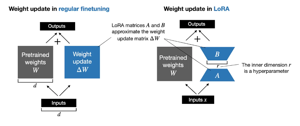
Fig. 5 Low-rank decomposition of the update weights \(\Delta \mathbf{W}\) into two matrices \(\mathbf{A}\) and \(\mathbf{B}\).#
Image Credit: Sebastian Raschka
First, we use very rough notations to describe the update weights of fine-tuning as a matrix \(\mathbf{W} \in \mathbb{R}^{d \times k}\) in a gradient-based optimization process. For simplicity we call \(\mathbf{W}\) as the pre-trained weights and \(\Delta \mathbf{W}\) as the update weights at a given iteration of a gradient-based optimization process. More concretely, we have the below update process:
where \(\mathcal{J}\) is the objective function, \(\alpha\) is the learning rate, and \(\nabla \mathbf{W}\) is the gradient of the objective function with respect to the pre-trained weights \(\mathbf{W}\) and collectively \(-\alpha \nabla \mathbf{W}\) is the update weights \(\Delta \mathbf{W}\) and that both \(\Delta \mathbf{W}\) and \(\nabla \mathbf{W}\) lies in the same subspace.
To ease the notations, we further denote \(\mathbf{W}^{(t)}\) as the pre-trained weights at iteration \(t\) and \(\Delta \mathbf{W}^{(t)}\) as the update weights at iteration \(t\). We can then rewrite the above equation as:
to indicate that \(\mathbf{W}^{(t+1)}\) is the updated weights after \(\Delta \mathbf{W}^{(t)}\) is added to the pre-trained weights \(\mathbf{W}^{(t)}\).
Empirical evidence suggests that deep learning models (often large language models) \(\mathcal{M}\) are over-parametrized with respect to their parameter space \(\Theta\) (i.e. the weights of the model). This means the model contains more parameters than are necessary to achieve the minimum error on the training data. This redundancy often implies that many parameters are either not essential or are correlated with others. While the “full space” offers maximal degrees of freedom for the model parameters, allowing complex representations and potentially capturing intricate patterns in the data, it can lead to overfitting, and in our context, it can lead to high computational costs and memory usage.
As a result, the authors hypothesize that \(\mathcal{M}\) can operate within a much lower-dimensional subspace \(\mathcal{S}\) which means that we can reduce the effective degrees of freedom of the model \(\mathcal{M}\) by projecting the weights of the model into a lower-dimensional subspace while maintaining the performance of the model - and this is what the author mean by “model resides in a low intrinsic dimension”.
More concretely, suppose the weight matrix \(\mathbf{W} \in \mathbb{R}^{d \times k}\) has rank \(r\) meaning the maximum number of linearly independent rows or columns it contains is \(r\). We say that this weight matrix reside in a subspace \(\mathcal{S}_{W} \subset \mathbb{R}^{d}\) (column space/range of \(\mathbf{W}\)) and the dimension of this subspace is \(r\). The authors argue that the update weights \(\Delta \mathbf{W}\) of the model \(\mathcal{M}\) at a given iteration of the optimization process also reside in a low-dimensional subspace \(\mathcal{S}_{\Delta \mathbf{W}} \subset \mathbb{R}^{d}\) with \(\dim\left(\mathcal{S}_{\Delta \mathbf{W}}\right) \ll r\). Note that without LoRA, the update weights \(\Delta \mathbf{W}\) typically have a high rank (not guaranteed to be of same rank of \(\mathbf{W}\)), and so the authors intelligently proposed an approximation of the update weights \(\Delta \mathbf{W}\) using a low-rank decomposition because of the hypothesis that the update weights reside in a low-dimensional subspace and is sufficient to represent the over-parametrized model \(\mathcal{M}\).
where \(\mathbf{A}^{(t)}\) and \(\mathbf{B}^{(t)}\) are the low-rank decomposition matrices of the update weights \(\Delta \mathbf{W}^{(t)}\) at iteration \(t\). In other words, the update weights \(\Delta \mathbf{W}\) are approximated by the product of two low-rank matrices \(\mathbf{A} \in \mathbb{R}^{r \times k}\) and and \(\mathbf{B} \in \mathbb{R}^{d \times r}\), where \(r \ll \min (d, k)\).
Parameters Reduction In LoRA#
Now, let’s do some quick math. Earlier we said our model is of size \(\| \Theta_{\mathcal{M}} \| = 175,000,000,000\) parameters. Then for simplicity case we assume our weight \(\mathbf{W} \in \mathbb{R}^{d \times k}\) of the pretrained model \(\mathcal{M}\) to be of size \(d = k = \sqrt{175,000,000,000} = 418,330\). And if we do not do LoRA, the update weights \(\nabla \mathbf{W}\) will also be of size \(d \times k = 418,330 \times 418,330 = 175,000,000,000\) parameters. However, if we decompose the update weights \(\nabla \mathbf{W}\) into two low-rank matrices \(\mathbf{A}\) and \(\mathbf{B}\), then the number of parameters in the low-rank decomposition is \(r \times (d + k)\). Suppose that we use a LoRA rank of \(r = 8\), then \(\mathbf{A} \in \mathbb{R}^{8 \times 418,330}\) and \(\mathbf{B} \in \mathbb{R}^{418,330 \times 8}\), and the number of parameters in the low-rank decomposition is \(8 \times (418,330 + 418,330) = 6,693,280\) parameters. We do some quick calculations and see that the reduction in the number of parameters is more than 26100 times.
 1import math
 2
 3def compute_lora_parameters(d: int, k: int, r: int) -> int:
 4    parameters_A = r * d
 5    parameters_B = r * k
 6    return parameters_A + parameters_B
 7
 8total_trainable_parameters = 175_000_000_000
 9print(f"Total trainable parameters: {total_trainable_parameters}")
10
11d = k = math.sqrt(total_trainable_parameters)
12r = 8
13lora_parameters = compute_lora_parameters(d, k, r)
14print(f"LoRA parameters: {lora_parameters}")
15
16reduction = (total_trainable_parameters - lora_parameters) / total_trainable_parameters
17print(f"Reduction: {reduction:.6%}")
18print(f"{total_trainable_parameters / lora_parameters}")
Total trainable parameters: 175000000000
LoRA parameters: 6693280.212272604
Reduction: 99.996175%
26145.625829189863
However, do note that there is no free lunch, we have to acknowledge that the rank \(r\) of the low-rank decomposition is a hyperparameter that needs to be tuned. Too small a rank can lead to underfitting, while too large a rank can lead to overfitting. Furthermore, no one knows the underlying “true” rank of the model and it may be well the case that the approximation \(\mathbf{B} \mathbf{A}\) is not a good approximation of the update weights \(\Delta \mathbf{W}\) and cannot capture every nuance. That is fine, for one, during pretraining stage, there is no low rank approximation and we hypothesize that the weight matrix \(\mathbf{W}\) is large and sufficient enough to capture all the nuances and knowledge in the huge pretraining dataset. However, during the fine-tuning stage, we hypothesize the domain specific task is not as complex as the pretraining task and that the model has sufficient knowledge to adapt to the domain specific task with a low-rank decomposition/approximation of the update weights \(\Delta \mathbf{W}\). This brings to our second point, if the target domain specific task \(\mathcal{T}\) is too drastically different from the pretraining task \(\mathcal{P}\), then the low-rank decomposition may not be able to capture the necessary information for the adaptation and the model may not perform well - so here we recommend increasing the rank \(r\) where appropriate.
The Low-Rank Adaptation (LoRA) Algorithm#
Let \(\mathcal{M}\) be our model with some linear layer with weights \(\mathbf{W} \in \mathbb{R}^{d \times k}\), where \(d\) is the output dimension and \(k\) is the input dimension (get used to this notation with PyTorch). In particular \(\mathbf{W}\) is the original pre-trained weights of the model \(\mathcal{M}\) (correspond to our \(\Theta_{\mathcal{P}}\) earlier).
import torch

torch.nn.Linear(in_features=8, out_features=16).weight.shape
>>> torch.Size([16, 8])
We define the linear transformation
\(f_{\mathbf{W}} : \mathbb{R}^k \rightarrow \mathbb{R}^d\) by
\(f_{\mathbf{W}}(\mathbf{x}) = \mathbf{x} @ \mathbf{W}^T\) where
\(\mathbf{x} \in \mathbb{R}^{1 \times k}\) (assume batch size of \(1\) for
simplicity). Note a quirk here is that we usually define the input as
\(\mathbb{R}^{\mathcal{B} \times k}\) where \(\mathcal{B}\) is the batch size and
transpose the weights from torch’s Linear layer.
import torch

torch.nn.Linear(in_features=8, out_features=16).weight.shape

x = torch.randn(1, 8)
x @ torch.nn.Linear(in_features=8, out_features=16).weight.T
Next, we define two low rank matrices \(\mathbf{A} \in \mathbb{R}^{r \times k}\) and \(\mathbf{B} \in \mathbb{R}^{d \times r}\) where \(r\) is the rank of the low-rank decomposition. We define transformations as:
For an input \(\mathbf{x} \in \mathbb{R}^k\), we technically have the following update:
But we have our pretrained model weights \(\mathbf{W}\) is frozen so we can compute the frozen output first as:
Why can we do this? Because of the distributive law of matrix multiplication. As we will mention again later, this allows the weight to be updated on the fly during inference, meaning we do not need to store the original pre-trained weights \(\mathbf{W}\) and only need to store the low-rank matrices \(\mathbf{A}\) and \(\mathbf{B}\) - which is much more tractable.
Then finally we have the following update:
However, three nuances here:
The pretrained weights \(\mathbf{W}\) of \(\mathcal{M}\) is frozen during training via
requires_grad=False. This tells PyTorch not to update the weights of the pretrained model during backpropagation. This is important because we want to keep the pretrained weights fixed and only update the low-rank matrices \(\mathbf{A}\) and \(\mathbf{B}\) - both of which are trainable.They use gaussian initialization for \(\mathbf{A}\) and zero initialization for \(\mathbf{B}\).
\[\begin{split} \begin{aligned} \mathbf{A} &\sim \mathcal{N}(0, \sigma^2) \\ \mathbf{B} &= \mathbf{0} \end{aligned} \end{split}\]One of the matrices must be zero at initialization to ensure that the initial state of the adaptation \(\Delta \mathbf{W}\) does not alter the pre-trained weights \(\mathbf{W}\), allowing the training process to start from the original pre-trained state. In simpler words, your first forward pass of the model should be from the original pre-trained weights \(\mathbf{W}\), and not from some random lora weights.
As to why \(\mathbf{A} \sim \mathcal{N}(0, \sigma^2)\), this is a common initialization strategy for neural networks to break the symmetry and ensure that the gradients are not too small or too large at the beginning of training. Just remember, vanishing and exploding gradients are bad, and we want to avoid them. How to avoid them is to make sure your initial conditions are good, what it means by good is say each layer weights has similar distribution (mean and variance) and so pertubations won’t be too large or too small. If you ask “if \(\mathbf{B} \mathbf{A}\) is zero, why don’t we just initialize \(\mathbf{A}\) to zero as well?” - I think one needs to know that the backpropagation process update both weights \(\mathbf{A}\) and \(\mathbf{B}\) separately and we want stable gradient flow, so \(\mathbf{A}\) breaks the symmetry! If you initialize all weights with zeros then every hidden unit will get zero independent of the input. So, when all the hidden neurons start with the zero weights, then all of them will follow the same gradient and for this reason “it affects only the scale of the weight vector, not the direction”. See this very useful thread on the whys.
They have a scaling factor, where they scale \(\Delta \mathbf{W}\) by \(\frac{\alpha}{r}\). In LoRA paper, \(\alpha\) is constant in \(r\) means that if once you fix a value of \(r\) in your initial experiments, you can keep \(\alpha\) constant for all future experiments with different values of \(r\) - because you can tune the learning rate scheduler’s \(\eta\) instead because yes both \(\alpha\) is pretty similar in scaling the gradients \(\nabla \mathbf{W}\) because by the chain rule, any scaling of the weights will proportionally affect the gradients! Note for less confusion, we use \(\eta\) for the learning rate in the optimizer and \(\alpha\) for the scaling factor in LoRA.
\[ \begin{aligned} \mathbf{y} &= \mathbf{y}_{\text{frozen}} + \frac{\alpha}{r} \mathbf{x} @ \left(\mathbf{B} \mathbf{A}\right)^T \end{aligned} \]Note that \(\alpha\) is generally understood as an amplification factor - and if \(\alpha\) is large, it amplifies the contribution of the LoRA weights to the final output of the adapter layer.
Now some quick and rough (read: non-rigorous) math here, suppose we keep rank \(r\) fixed, and we increase \(\alpha\) (LoRA) by a factor of \(c\):
\[\begin{split} \begin{aligned} c \times \frac{\alpha}{r} \mathbf{x} @ \left(\mathbf{B} \mathbf{A}\right)^T &= (c \times \eta) \times \mathbf{x} @ \left(\frac{\mathbf{B}}{\sqrt{c}} \frac{\mathbf{A}}{\sqrt{c}}\right)^T \\ \end{aligned} \end{split}\]So in other words, if you keep \(r\) fixed, when you increase \(\alpha\) by a factor of \(c\) - this is equivalent to increasing the learning rate \(\eta\) by a factor of \(c\) because in gradient updates we do \(-\eta \nabla \left(\mathbf{B}\mathbf{A}\right)\) and so if you increase \(\alpha\) by a factor of \(c\), you are inevitably increasing the learning rate \(\eta\) by a factor of \(c\). To compensate for this, you can decrease the initializations of \(\mathbf{A}\) and \(\mathbf{B}\) by a factor of \(\sqrt{c}\) to keep to the same scale as before. Therefore, the authors recommend users to (1) keep the rank \(r\) fixed and (2) tune the learning rate scheduler’s \(\eta\) instead of \(\alpha\) (and maybe the weights as well). One can read a thread on this here.
Merge - No Additional Inference Latency#
The distributive law of matrix multiplication we saw earlier ensures that the update weights \(\Delta \mathbf{W}\) can be applied on the fly during inference without too much over memory overhead, and therefore not much additional latency. Recall the equation below:
We easily see that once we obtain the trained low-rank matrices \(\mathbf{A}\) and \(\mathbf{B}\), we can apply the update weights \(\Delta \mathbf{W}\) on the fly during inference without having to store the original pre-trained weights by just doing an element-wise addition of the frozen output \(\mathbf{y}_{\text{frozen}}\) and the update \(\mathbf{x} @ \left(\mathbf{B} \mathbf{A}\right)^T\).
Again, we are reminded that this is a huge advantage because we need not store \(N\) instances of the updated weights \(\Delta \mathbf{W}\) for \(N\) different tasks, but only the low-rank matrices \(\mathbf{A}\) and \(\mathbf{B}\). During inference, just apply the low-rank matrices on the fly and you are good to go.
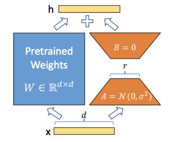
Fig. 6 LoRA update weights \(\Delta \mathbf{W}\) as a low-rank decomposition of two matrices \(\mathbf{A}\) and \(\mathbf{B}\).#
Image Credit: LoRA Paper
In practice, it is common to merge and unload the adapter layer after training into the original pretrained base model. This merge operation is done by updating the original pretrained weights \(\mathbf{W}\) with the low-rank decomposition matrices \(\mathbf{A}\) and \(\mathbf{B}\) to obtain the merged weights \(\mathbf{W}_{'}\).
This way, during inference, given an input \(\mathbf{x}\), we can compute the output \(\mathbf{y}\) by applying the merged weights \(\mathbf{W}^{'}\) on the input \(\mathbf{x}\).
This requires only a single matrix multiplication operation. In total, we can loosely say that if \(\mathbf{x}\) is a \(1 \times k\) vector, and \(\mathbf{W}^{'} \in \mathbb{R}^{d \times k}\), then doing \(\mathbf{x} @ \left(\mathbf{W}^{'}\right)^T\) costs \(2 \times d \times k\) multiplications and \(d \times k\) additions. But if you do not merge, and keep the weights separate, you get \(\mathbf{x} @ \left(\mathbf{W}^T\right) + \mathbf{x} @ \left(\mathbf{B} \mathbf{A}\right)^T\) which costs \(2 \times d \times k\) multiplications and \(2 \times d \times k\) additions. So, in terms of computational complexity, even though they are on the same order, the merged weights are slightly more efficient.
References And Further Readings#
[1] E. J. Hu, Y. Shen, P. Wallis, Z. Allen-Zhu, Y. Li, S. Wang, L. Wang, and W. Chen, “LoRA: Low-Rank Adaptation of Large Language Models,” arXiv preprint arXiv:2106.09685, submitted Jun. 17, 2021, revised Oct. 16, 2021. [Online]. Available: https://arxiv.org/abs/2106.09685
[2] A. Vaswani, N. Shazeer, N. Parmar, J. Uszkoreit, L. Jones, A. N. Gomez, Ł. Kaiser, and I. Polosukhin. “Attention is all you need”. In Advances in Neural Information Processing Systems, pp. 5998–6008, 2017.