Stage 9. Model Monitoring (MLOps)#
Model monitoring is about continuously tracking the performance of models in production to ensure that they continue to provide accurate and reliable predictions.
Performance Monitoring: Regularly evaluate the model’s performance metrics in production. This includes tracking metrics like accuracy, precision, recall, F1 score for classification problems, or Mean Absolute Error (MAE), Root Mean Squared Error (RMSE) for regression problems, etc.
Data Drift Monitoring: Over time, the data that the model receives can change. These changes can lead to a decrease in the model’s performance. Therefore, it’s crucial to monitor the data the model is scoring on to detect any drift from the data the model was trained on.
Model Retraining: If the performance of the model drops or significant data drift is detected, it might be necessary to retrain the model with new data. The model monitoring should provide alerts or triggers for such situations.
A/B Testing: In case multiple models are in production, monitor their performances comparatively through techniques like A/B testing to determine which model performs better.
In each of these stages, it’s essential to keep in mind principles like reproducibility, automation, collaboration, and validation to ensure the developed models are reliable, efficient, and providing value to the organization.
Intuition#
Even though we’ve trained and thoroughly evaluated our model, the real work begins once we deploy to production. This is one of the fundamental differences between traditional software engineering and ML development. Traditionally, with rule-based, deterministic software, the majority of the work occurs at the initial stage and once deployed, our system works as we’ve defined it. But with machine learning, we haven’t explicitly defined how something works but used data to architect a probabilistic solution. This approach is subject to natural performance degradation over time, as well as unintended behavior, since the data exposed to the model will be different from what it has been trained on. This isn’t something we should be trying to avoid but rather understand and mitigate as much as possible. In this lesson, we’ll understand the shortcomings from attempting to capture performance degradation in order to motivate the need for drift detection.
System Health#
The first step to ensure that our model is performing well is to ensure that the actual system is up and running as it should. This can include metrics specific to service requests such as latency, throughput, error rates, etc. as well as infrastructure utilization such as CPU/GPU utilization, memory, etc.
Service Metrics:
Latency: Time taken to process requests.
Throughput: Number of requests processed per unit time.
Error Rates: Frequency of failed requests.
Infrastructure Metrics:
CPU/GPU Utilization: Resource usage of the hardware.
Memory Consumption: Amount of memory used by the system.
Fortunately, most cloud providers and even orchestration layers will provide this insight into our system’s health for free through a dashboard. In the event we don’t, we can easily use Grafana, Datadog, etc. to ingest system performance metrics from logs to create a customized dashboard and set alerts. If you use AWS for example, you can use AWS CloudWatch to monitor your system’s health.
Categorizing Drift Types#
We use a table from madewithml to illustrate the different types of drift.
Data Drift#
Objective: Detect changes in the input data distribution that may affect model performance.
Approach: Compare the distribution of incoming data with the data used during training.
Techniques: Statistical tests (e.g., t-tests), visualization (e.g., histograms), drift detection algorithms.
Concept Drift#
Objective: Identify changes in the relationship between input features and the target variable.
Indicator: Decline in model performance without significant data drift.
Action: Retrain or adjust the model to accommodate new underlying patterns.
Sometimes, even if the data distribution stays the same, the underlying relationship between the input features and the target variable might change. This is called concept drift. To monitor this, you can look for a decrease in your model’s performance over time, even when there’s no significant data drif
Let’s consider a concrete example of concept drift in the context of a movie recommendation system.
Suppose you have a movie recommendation algorithm that takes into account factors like user’s age, genre preferences, and ratings of previously watched movies to recommend new movies. The model is trained on a dataset and works well initially, giving good recommendations and having a high click-through rate.
Over time, however, you notice that even though the distribution of the user’s age, genre preferences, and ratings of previously watched movies (your input features) stays the same, the click-through rate of the recommended movies (your target variable) starts to decrease. This indicates that the relationship between the input features and the target variable has changed.
Why might this happen? One possible reason is a change in movie trends. Perhaps when the model was initially trained, action movies were very popular. But over time, the popularity of action movies has decreased and documentaries have become more popular. The model, however, is still biased towards recommending action movies because that’s what worked when it was initially trained. This is an example of concept drift: the underlying concept – what kind of movies are likely to be clicked on – has changed, even though the distribution of the input features has not.
To monitor this, you would track the performance of your model over time. If you see a decrease in performance – in this case, a decrease in the click-through rate – that could be an indication of concept drift. You might then decide to retrain your model on more recent data, or to revise it to take into account more recent trends in movie popularity.
Target Drift#
Objective: Detect changes in the target variable distribution.
Approach: Compare the distribution of the target variable in the incoming data with the distribution used during training.
Techniques: Statistical tests (e.g., t-tests), visualization (e.g., histograms), drift detection algorithms.
Example: Monitoring a Bitcoin Price Prediction Model#
To illustrate model and data drift monitoring, let’s consider a Bitcoin price prediction model. Here’s how to systematically monitor and maintain its performance:
1. Model Performance Monitoring#
Metrics to Track:
Regression Metrics: MAE, RMSE, \(R^2\) Score.
Procedure:
Evaluate these metrics at regular intervals (e.g., daily, weekly).
Plot metrics over time to identify trends or sudden changes.
Action:
If metrics degrade beyond acceptable thresholds, initiate model retraining or adjustments.
2. Data Drift Monitoring#
Objective: Ensure that the input data distribution remains similar to the training data.
Method: Use statistical tests to compare distributions of incoming data with reference data.
Using Two-Sample t-Tests for Data Drift#
Steps:
Select Features: Focus on individual features (e.g., ‘Volume’, ‘Open’, ‘Close’).
Sample Data:
Current Data: Collect a sample from the incoming data stream.
Reference Data: Use a sample from the original training dataset.
Compute Statistics:
Calculate the mean (
mean1) and standard deviation (std1) for the current data.Calculate the mean (
mean2) and standard deviation (std2) for the reference data.
Perform t-Test:
Compute the t-score using the formula:
\[ t = \frac{\text{mean1} - \text{mean2}}{\sqrt{\frac{\text{std1}^2}{n1} + \frac{\text{std2}^2}{n2}}} \]where \(n1\) and \(n2\) are sample sizes.
Interpret Results:
Compare the absolute t-score with the critical t-value for the desired confidence level.
A large absolute t-score indicates a significant difference in means, suggesting data drift.
Frequency: Conduct these tests for all relevant features at regular intervals (e.g., daily, weekly).
3. Concept Drift Monitoring#
Objective: Detect changes in the relationship between input features and the target variable.
Indicator: A decline in model performance without significant data drift.
Monitoring Dashboard In Practice#
A hands on example of how to monitor a model’s performance using Kibana can be found in this MLOps Basics [Week 9]: Prediction Monitoring - Kibana blog post.
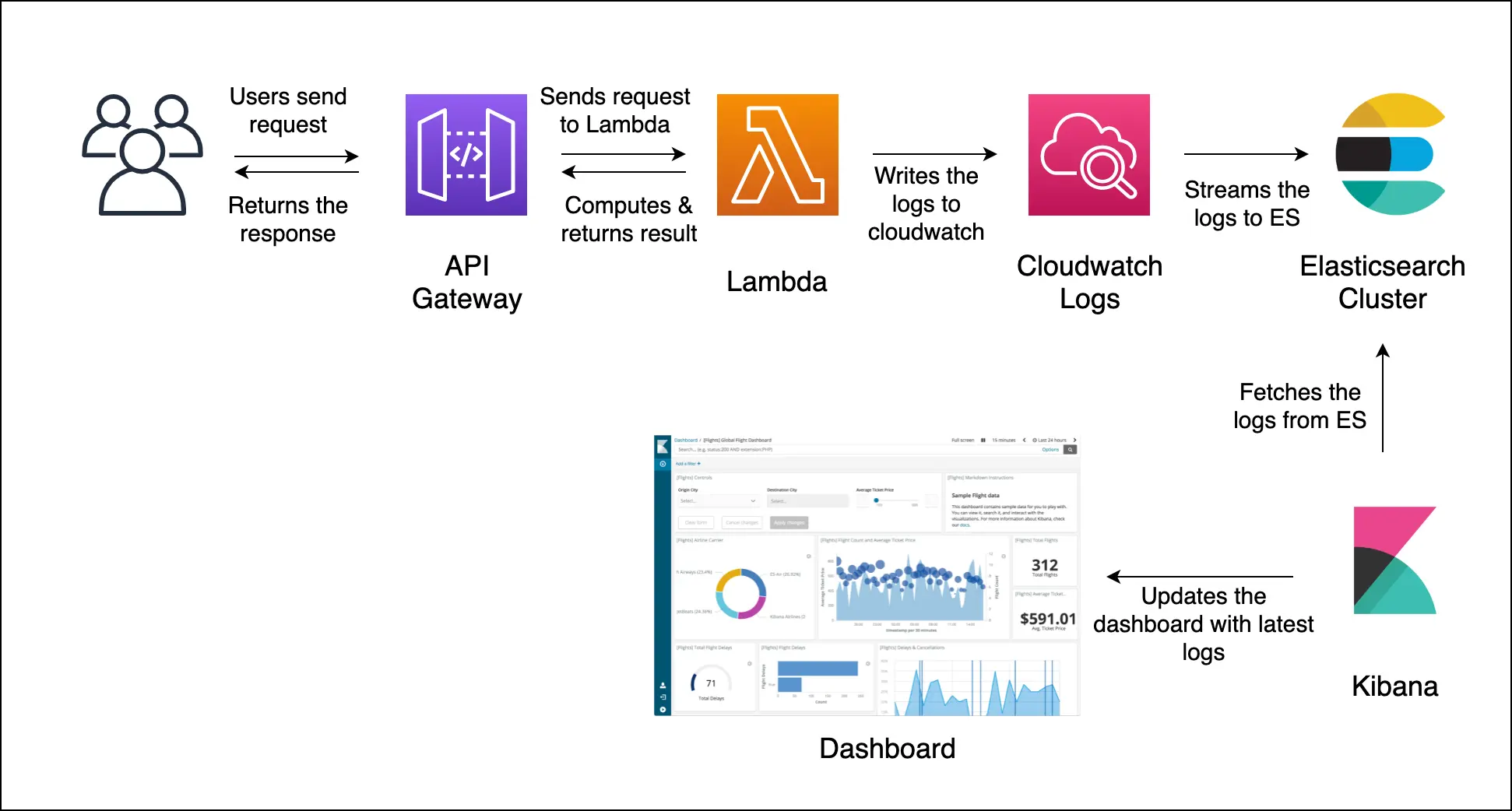
Fig. 53 Kibana flow.#
Image Credits: MLOps Basics [Week 9]: Prediction Monitoring - Kibana
References and Further Readings#
Huyen, Chip. “Chapter 8. Data Distribution Shifts and Monitoring.” In Designing Machine Learning Systems: An Iterative Process for Production-Ready Applications, O’Reilly Media, Inc., 2022.