Gaussian Distribution#
Perhaps the most important distribution is the Gaussian Distribution, also known as the Normal Distribution.
General Gaussian Distribution#
Definition#
Definition 119 (Gaussian Distribution (PDF))
\(X\) is a continuous random variable with a Gaussian distribution if the probability density function is given by:
where \(\mu\) is the mean and \(\sigma^2\) is the variance and are parameters of the distribution.
Some conventions:
We write \(X \sim \gaussian(\mu, \sigma^2)\) to indicate that \(X\) has a Gaussian distribution with mean \(\mu\) and variance \(\sigma^2\).
We sometimes denote \(\gaussian\) as \(\normal\) or \(\gaussiansymbol\).
Definition 120 (Gaussian Distribution (CDF))
There is no closed form for the CDF of the Gaussian distribution. But we will see that it is easy to compute the CDF of the Gaussian distribution using the CDF of the standard normal distribution later.
Therefore, the CDF of the Gaussian distribution is given by:
Yes, you have to integrate the PDF to get the CDF but there is no “general” solution.
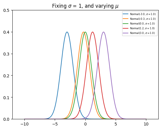
The PDF of the Gaussian distribution is shown below. The code is referenced and modified from [Shea, 2021].
<>:20: SyntaxWarning: invalid escape sequence '\s'
<>:26: SyntaxWarning: invalid escape sequence '\s'
<>:44: SyntaxWarning: invalid escape sequence '\s'
<>:50: SyntaxWarning: invalid escape sequence '\m'
<>:20: SyntaxWarning: invalid escape sequence '\s'
<>:26: SyntaxWarning: invalid escape sequence '\s'
<>:44: SyntaxWarning: invalid escape sequence '\s'
<>:50: SyntaxWarning: invalid escape sequence '\m'
/tmp/ipykernel_3758/3973853284.py:20: SyntaxWarning: invalid escape sequence '\s'
label = f"Normal({N.mean()}, $\sigma=${N.std() :.1f})"
/tmp/ipykernel_3758/3973853284.py:26: SyntaxWarning: invalid escape sequence '\s'
plt.title("Fixing $\sigma$ = 1, and varying $\mu$")
/tmp/ipykernel_3758/3973853284.py:44: SyntaxWarning: invalid escape sequence '\s'
label = f"Normal({N.mean()}, $\sigma=${N.std() :.1f})"
/tmp/ipykernel_3758/3973853284.py:50: SyntaxWarning: invalid escape sequence '\m'
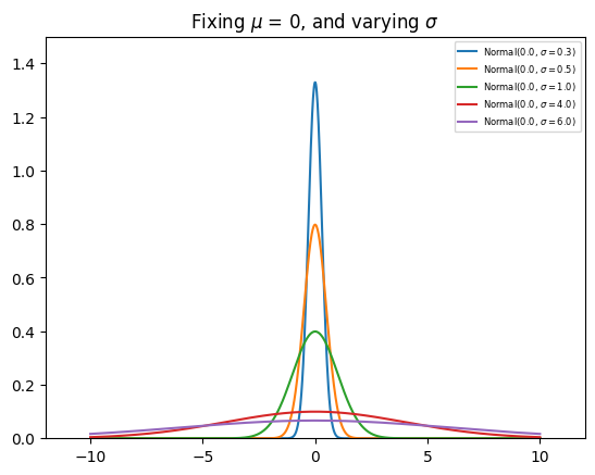
plt.title("Fixing $\mu$ = 0, and varying $\sigma$")
Remark 47 (Gaussian Distribution (PDF))
Note in the plots above, the PDF of the Gaussian distribution is symmetric about the mean \(\mu\), and given a small enough \(\sigma\), the PDF can be greater than 1, as long as the area under the curve is 1.
Note that the PDF curve moves left and right as \(\mu\) increases and decreases, respectively. Similarly, the PDF curve gets narrower and wider as \(\sigma\) increases and decreases, respectively.
Expectation and Variance#
Theorem 30 (Expectation and Variance of the Gaussian Distribution)
The observant reader may notice that the mean and variance of the Gaussian distribution are parameters of the distribution. However, this is not proven previously.
If \(X\) is a continuous random variable with an gaussian distribution with mean \(\mu\) and variance \(\sigma^2\), then the expectation and variance of \(X\) are given by:
Linear Transformation of Gaussian Distribution#
Theorem 31 (Linear Transformation of Gaussian Distribution)
Let \(X \sim \gaussiansymbol(\mu, \sigma^2)\) be a random variable with a Gaussian distribution with mean \(\mu\) and variance \(\sigma^2\).
Let \(Y = aX + b\) be a linear transformation of \(X\).
Then, \(Y \sim \gaussiansymbol(a\mu + b, a^2\sigma^2)\) is a Gaussian distribution with mean \(a\mu + b\) and variance \(a^2\sigma^2\).
In other words, \(Y\) experiences a shift and scale change in coordinates, and while the distribution may not longer be the same as \(X\), it still belongs to the same family.
Standard Gaussian Distribution#
Motivation#
In continuous distributions, we are often asked to evaluate the probability of an interval \([a, b]\). For example, if \(X \sim \gaussian(\mu, \sigma^2)\), what is the probability that \(X\) is between \(a\) and \(b\)? If we use PDF to compute the probability, we will have to integrate the PDF over the interval \([a, b]\).
We have seen that there is no closed form solution for this integral.
Furthermore, in practice, we use the CDF to compute the probability of an interval.
However, we have also seen that there is no closed form solution for the CDF of the Gaussian distribution since the CDF is an integral of the PDF.
This prompted the existence of the standard normal distribution.
Definition#
Definition 121 (Standard Gaussian Distribution)
Let \(X\) be a continuous random variable with a Gaussian distribution with mean \(\mu\) and variance \(\sigma^2\). Then \(X\) is said to be a Standard Gaussian if it has a Gaussian distribution with mean 0 and variance 1.
In notations, it is \(X \sim \gaussiansymbol(0, 1)\), with \(\mu = 0\) and \(\sigma^2 = 1\).
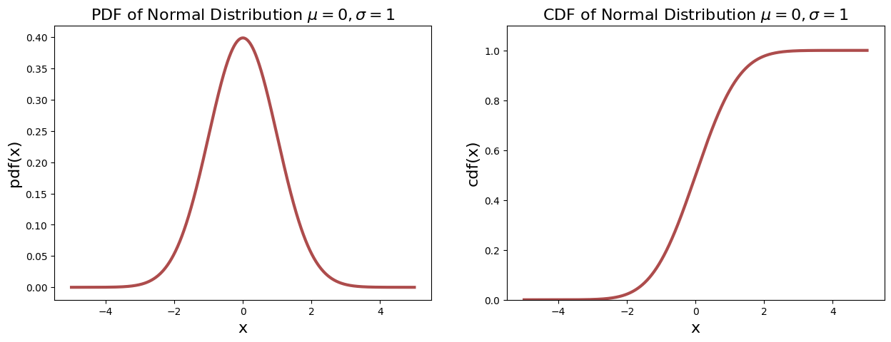
Definition 122 (Standard Normal Distribution (CDF))
The CDF of the Standard Gaussian is given by:
Take note of the \(\Phi\) notation, which is the standard notation for the CDF of the Standard Gaussian.
<>:17: SyntaxWarning: invalid escape sequence '\m'
<>:17: SyntaxWarning: invalid escape sequence '\m'
/tmp/ipykernel_3758/2820111295.py:17: SyntaxWarning: invalid escape sequence '\m'
  plot_continuous_pdf_and_cdf(X, -5, 5, title="Normal Distribution $\mu=0, \sigma=1$", figsize=(15, 5))
Error Function#
Definition 123 (Error Function)
The error function is defined as:
The connection of the error function to the CDF of the Standard Gaussian is given by:
CDF of Arbitrary Gaussian Distribution#
Theorem 32 (CDF of Arbitrary Gaussian Distribution)
Let \(X\) be a continuous random variable with a Gaussian distribution with mean \(\mu\) and variance \(\sigma^2\). Then we can convert the CDF of \(X\) to the CDF of the Standard Gaussian by:
Proof. CDF of Arbitrary Gaussian Distribution The definition of a Gaussian distribution is given by:
We can use the (integration by) substitution \(u = \frac{t - \mu}{\sigma}\) to get [Chan, 2021]:
Corollary 8 (Probability of an Interval)
As a consequence of Theorem 32, we can compute the probability of an interval for an arbitrary Gaussian distribution. This solves our problem of computing the probability of an interval for a Gaussian Distribution earlier.
Corollary 9 (Corollary of Standard Gaussian)
As a consequence of Theorem 32, we have the following corollaries [Chan, 2021]:
\(\Phi(y) = 1 - \Phi(-y)\)
\(\P \lsq X \geq b \rsq = 1 - \Phi \lpar \frac{b - \mu}{\sigma} \rpar\)
\(\P \lvert X \rvert \geq b = 1 - \Phi \lpar \frac{b - \mu}{\sigma} \rpar + \Phi \lpar \frac{-b - \mu}{\sigma} \rpar\)
References and Further Readings#
Chan, Stanley H. “Chapter 4.6. Gaussian Random Variables.” In Introduction to Probability for Data Science, 211-223. Ann Arbor, Michigan: Michigan Publishing Services, 2021.
Pishro-Nik, Hossein. “Chapter 4.2.3. Normal (Gaussian) Distribution” In Introduction to Probability, Statistics, and Random Processes, 253-260. Kappa Research, 2014.