Notations#
To simplify notations, we assume that each node has the same number of GPUs so that we can have less indexes to keep track of. In particular, we assume the following notations. We can refer to CS336 for more information.
Process#
\(P\) (Worker/Number of Processes): is the number of processes across the cluster of nodes;
\(p\): is the index of a process, \(p \in [0, P)\);
A process is a program in execution, characterized by a unique process ID and its own independent set of system resources. It possesses its own memory space, including code, runtime memory, and system resources. Processes are isolated from each other, ensuring that the actions (or failures) of one process don’t directly affect another. They can communicate with each other through various inter-process communication mechanisms.
It is an instance of a program that’s participating in the distributed training. In this assignment, each worker will have a single process, so we’ll use worker, process, and worker process interchangeably. However, a worker may use multiple processes (e.g., to load data for training), so these terms are not always equivalent in practice.
In the context of distributed computing and deep learning, a process typically refers to an instance of a training algorithm running on a computational unit (like a CPU core or GPU).
Nodes#
\(N\) (Number of Nodes): is the number of nodes in the cluster;
\(n\): is the index of a node in the cluster, \(n \in [0, N)\);
A node is a physical machine with its own operating system and system resources. It can have multiple CPUs and GPUs. For example,
g4dn.4xlargeis a node type in AWS EC2 that has 2 GPUs.
Local And Global World Size#
\(G\) (Local World Size): is the number of GPUs per node or the number of processes per node or local world size;
\(g\): is the index of a GPU in a node, \(g \in [0, G)\);
A GPU is a computational unit that can perform parallel computation on tensors. It has its own memory space, including code, runtime memory, and system resources. Consequently, we often collapse the notion of a GPU and a process together, and use the two terms interchangeably.
\(W\): is the world size;
The world size refers to the total number of application processes \(P\) running across the cluster of nodes \(N\). So \(W = P\).
Since in the context of distributed deep learning training, the process and the GPU are often used interchangeably where each GPU runs one process , we can also say that the world size \(W\) is the total number of GPUs across the cluster of nodes \(N\).
\[ W = N \times G \]
Local And Global Rank#
Global Rank (often denoted just as Rank) \(R_g \in [0, W-1]\): is the global rank of a process across the cluster of nodes;
\(R_g = n \times G + g\) where \(n\) is the index of a node and \(g\) is the index of a GPU in that particular node \(n\);
The global rank \(R_g\) is the unique identifier of a process across the cluster of nodes. It is used to identify a process in the collective communication operations.
In the context of distributed deep learning training, the global rank \(R_g\) is the unique identifier of a GPU across the cluster of nodes. It is used to identify a GPU in the collective communication operations.
Local Rank \(R_{l} \in [0, L-1]\): is the local rank of a process within a node;
\(R_{l} = g\);
The local rank \(R_{l}\) is the unique identifier of a process within a node. It is used to identify a process in the intra-node collective communication operations.
In the context of distributed deep learning training, the local rank \(R_l\) is the unique identifier of a GPU within a node. It is used to identify a GPU in the intra-node collective communication operations.
An Example To Illustrate The Notations#
To illustrate the terminology defined above, consider the case where a DDP application is launched on two nodes, each of which has four GPUs. We would then like each process to span one GPUs each. The mapping of processes to nodes is shown in the figure below:

Fig. 36 2 nodes with 4 GPUs each and each process spans 1 GPU.#
More concretely, we have the following notations:
\(N = 2\): the number of nodes in the cluster;
\(G = 4\): the number of GPUs per node;
\(W = N \times G = 8\): the world size, i.e., the total number of GPUs across the cluster of nodes;
Now in node \(n=0\), we have the following notations:
GPU \(0\) corresponds to \(R_g = 0\) and \(R_l = 0\);
GPU \(1\) corresponds to \(R_g = 1\) and \(R_l = 1\);
GPU \(2\) corresponds to \(R_g = 2\) and \(R_l = 2\);
GPU \(3\) corresponds to \(R_g = 3\) and \(R_l = 3\);
The local ranks of the processes in node \(n=0\) are \(R_{l} \in [0, 3]\);
The global ranks of the processes in node \(n=0\) are \(R_{g} \in [0, 3]\);
Now in node \(n=1\), we have the following notations:
GPU \(0\) corresponds to \(R_g = 4\) and \(R_l = 0\);
GPU \(1\) corresponds to \(R_g = 5\) and \(R_l = 1\);
GPU \(2\) corresponds to \(R_g = 6\) and \(R_l = 2\);
GPU \(3\) corresponds to \(R_g = 7\) and \(R_l = 3\);
The local ranks of the processes in node \(n=1\) are \(R_{l} \in [0, 3]\);
The global ranks of the processes in node \(n=1\) are \(R_{g} \in [4, 7]\);
To illustrate the terminology defined above, consider the case where a DDP application is launched on two nodes, each of which has four GPUs. We would then like each process to span two GPUs each. The mapping of processes to nodes is shown in the figure below:
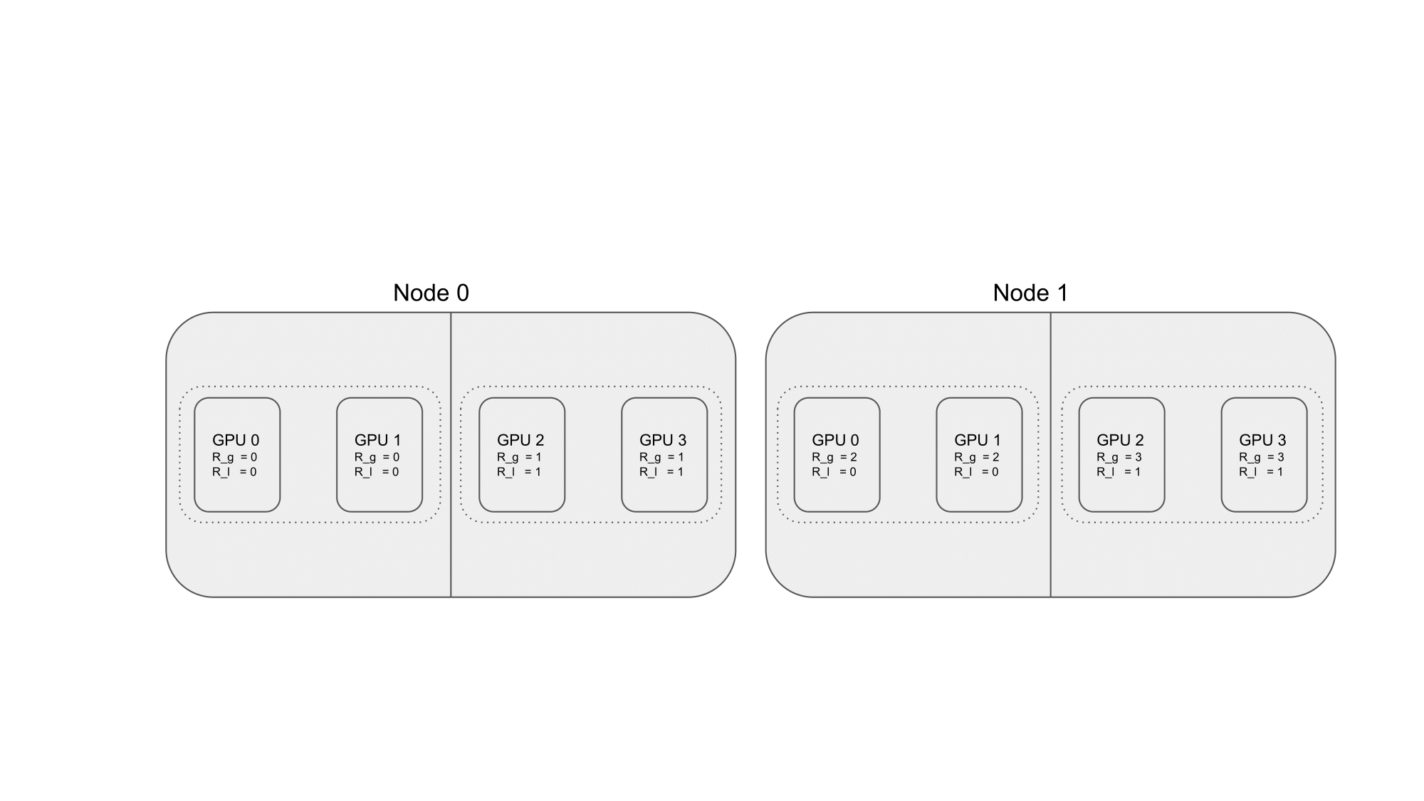
Fig. 37 2 nodes with 4 GPUs each and each process spans 2 GPUs.#
More concretely, for this scenario:
\(N = 2\): the number of nodes in the cluster.
\(G = 4\): the number of GPUs per node.
Since each process spans two GPUs, we will have half the number of processes compared to GPUs in each node. Let’s call the number of processes in each node \(P_{node}\).
\(P_{node} = \frac{G}{2} = 2\): number of processes per node.
\(W = N \times P_{node} = 4\): the world size, i.e., the total number of processes across the cluster of nodes.
For node \(n=0\):
Process \(0\) spans GPU \(0\) and GPU \(1\):
Global rank: \(R_g = 0\)
Local rank: \(R_l = 0\)
Process \(1\) spans GPU \(2\) and GPU \(3\):
Global rank: \(R_g = 1\)
Local rank: \(R_l = 1\)
The local ranks of the processes in node \(n=0\) are \(R_{l} \in [0, 1]\).
The global ranks of the processes in node \(n=0\) are \(R_{g} \in [0, 1]\).
For node \(n=1\):
Process \(2\) spans GPU \(0\) and GPU \(1\):
Global rank: \(R_g = 2\)
Local rank: \(R_l = 0\)
Process \(3\) spans GPU \(2\) and GPU \(3\):
Global rank: \(R_g = 3\)
Local rank: \(R_l = 1\)
The local ranks of the processes in node \(n=1\) are \(R_{l} \in [0, 1]\).
The global ranks of the processes in node \(n=1\) are \(R_{g} \in [2, 3]\).
In this scenario, while the number of GPUs in each node remains unchanged, the concept of process has been expanded to span two GPUs. This implies that the computation associated with each process is now distributed across two GPUs on the same node. Such a configuration can be useful for models that are too large to fit in the memory of a single GPU or for scenarios where inter-GPU communication within the same node is more efficient than across nodes.