Chapter 8. Estimation Theory

Table of Contents

• Maximum Likelihood Estimation

Consider the common machine learning setup for a classification problem with \(K\) classes, \(k \geq 1\).

Let \(\mathcal{P}_{\mathcal{D}}\) (denoted as \(\mathcal{D}\) usually) be the underlying probability distribution over some input space \(\mathcal{X}\) and output space \(\mathcal{Y} = \{1, \ldots, K\}\).

The learner receives a dataset \(\mathcal{S}\) with \(N\) samples, denoted as:

\[ \mathcal{S} = \left\{\mathbf{x}^{(i)}, y^{(i)}\right\}_{i=1}^{N} \in \left(\mathcal{X} \times \mathcal{Y}\right)^{N} \]

which are drawn indepedently and identically distributed (i.i.d.) from \(\mathcal{P}_{\mathcal{D}}\).

This typical setup abstracts away something very important due to notation simplicity. In reality, we can denote the underlying distribution as follows:

\[ \mathbb{P}_{\mathcal{D}}\left(\mathcal{X}, \mathcal{Y};\boldsymbol{\theta}\right) , \]

where \(\boldsymbol{\theta}\) is a parameter that characterizes the distribution \(\mathcal{P}_{\mathcal{D}}\).

Since \(\mathbb{P}_{\mathcal{D}}\left(\mathcal{X}, \mathcal{Y};\boldsymbol{\theta}\right)\) is unknown to us, it follows that \(\boldsymbol{\theta}\) is also unknown to us. Consequently, the whole goal of estimation is to solve an inverse problem to recover the parameter \(\boldsymbol{\theta}\) based on the observations in \(\mathcal{S}\).

Let’s see this pictorially:

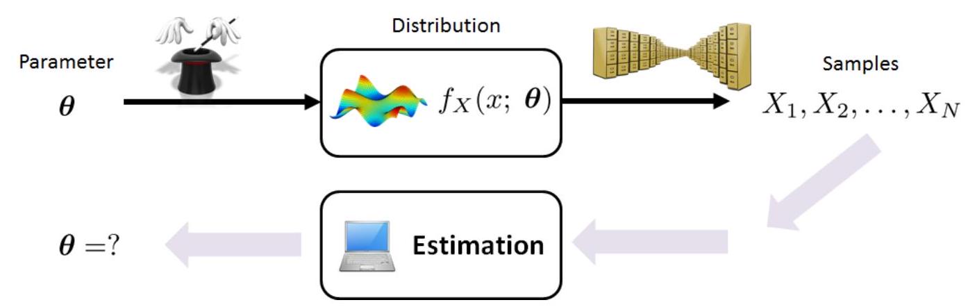
Fig. 34 Estimation is an inverse problem of recovering the unknown parameters that were used by the distribution. In this figure, the PDF of \(X\) using a parameter \(\boldsymbol{\theta}\) is denoted as \(f_{X}(x ; \boldsymbol{\theta})\). The forward data-generation process takes the parameter \(\boldsymbol{\theta}\) and creates the random samples \(X^{(1)}, \ldots, X^{(N)}\). Estimation takes these observed random samples and recovers the underlying model parameter \(\boldsymbol{\theta}\). Image Credit: [Chan, 2021].

Parameters

In the previous section, we introduced the concept of a parameter \(\boldsymbol{\theta}\) that characterizes the distribution \(\mathcal{P}_{\mathcal{D}}\).

The definition of parameters can be made more apparent with some examples, all of which adapted from [Chan, 2021].

Example 39 (Parameter of a Bernoulli Distribution)

If \(x^{(n)}\) is a Bernoulli random variable, then the PMF has a parameter \(\theta\) :

\[ p_{x^{(n)}}\left(x^{(n)} ; \theta\right)=\theta^{x^{(n)}}(1-\theta)^{1-x^{(n)}} \]

Remark. The PMF is expressed in this form because \(x^{(n)}\) is either 1 or 0 :

\[\begin{split} p_{x^{(n)}}\left(x^{(n)} ; \theta\right)=\left\{\begin{array}{lll} \theta^{1}(1-\theta)^{1-1}=\theta, & \text { if } & x^{(n)}=1, \\ \theta^{0}(1-\theta)^{1-0}=1-\theta, & \text { if } & x^{(n)}=0 \end{array}\right. \end{split}\]

Example 40 (Parameter of a Gaussian Distribution)

If \(x^{(n)}\) is a Gaussian random variable, the \(\mathrm{PDF}\) is

\[ f_{x^{(n)}}(x^{(n)} ; \underbrace{\boldsymbol{\theta}}_{=(\mu, \sigma)})=\frac{1}{\sqrt{2 \pi \sigma^{2}}} \exp \left\{-\frac{\left(x^{(n)}-\mu\right)^{2}}{2 \sigma^{2}}\right\} \]

where \(\boldsymbol{\theta}=[\mu, \sigma]\) consists of both the mean and the variance. We can also designate the parameter \(\theta\) to be the mean only. For example, if we know that \(\sigma=1\), then the \(\mathrm{PDF}\) is

\[ f_{x^{(n)}}(x^{(n)} ; \underbrace{\theta}_{=\mu})=\frac{1}{\sqrt{2 \pi}} \exp \left\{-\frac{\left(x^{(n)}-\mu\right)^{2}}{2}\right\} \]

where \(\theta\) is the mean.

Good and Bad Estimates

The estimation problem is well defined, let’s see some pictorial examples below in Fig. 35.

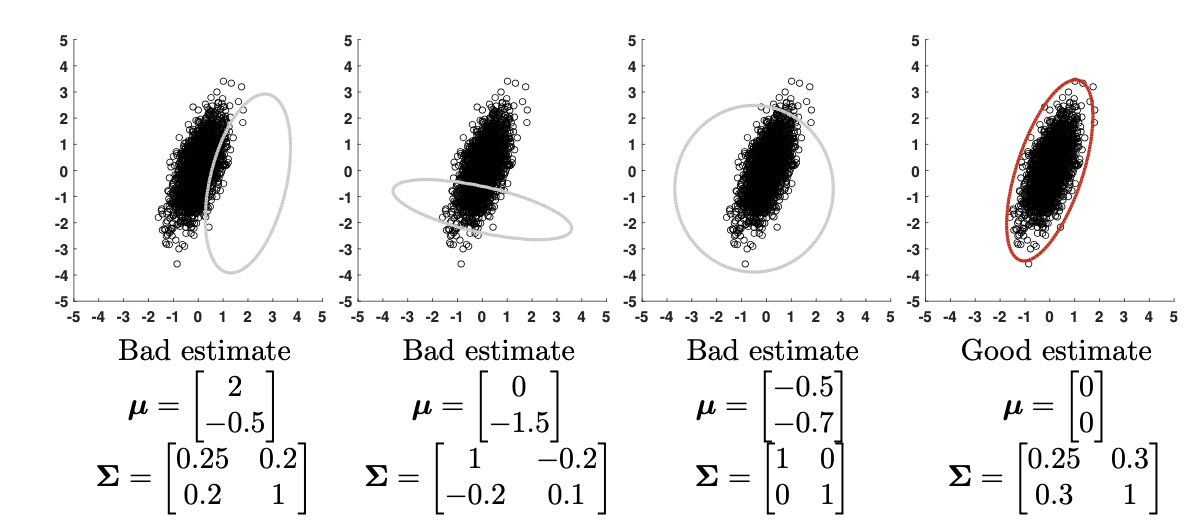
Fig. 35 Image Credit: [Chan, 2021].

The figure shows a dataset containing 1000 data points generated from a 2D Gaussian distribution with an unknown mean vector \(\boldsymbol{\mu}\) and an unknown covariance matrix \(\boldsymbol{\Sigma}\). We duplicate this dataset in the four subfigures. The estimation problem is to recover the unknown mean vector \(\boldsymbol{\mu}\) and the covariance matrix \(\boldsymbol{\Sigma}\). In the subfigures we propose four candidates, each with a different mean vector and a different covariance matrix. We draw the contour lines of the corresponding Gaussians. It can be seen that some Gaussians fit the data better than others (i.e. pictorially the right most predicted Gaussian is the best fit). The goal of this chapter is to develop a systematic way of finding the best fit for the data [Chan, 2021].

Notations

In what follows, we may at some parts drop the labels \(y\) and only focus on the input \(\mathbf{x}\).

We also adopt the notations described in this section for this chapter.