Stage 8. Model Serving (MLOps)#
Model serving is the process of making the trained machine learning models available for inference. It involves loading the model into memory and setting up an API or a service to accept data inputs, perform predictions, and return the results.
Deployment: Models are deployed in a suitable environment that can be a server, a cloud service, or even an edge device. Depending on the use case, the deployment can be a batch scoring job that runs at regular intervals, or a real-time scoring service that needs to respond immediately to incoming requests.
Scalability: The model serving infrastructure should be able to handle varying loads. It should be able to scale up during high load times and scale down when the load is low to efficiently use resources.
Latency: For real-time applications, the model serving infrastructure should have low latency to deliver predictions within an acceptable time frame.
Finite vs. Unbounded Feature Space, Precurser to Deployment Strategies#
The concept of finite vs. unbounded feature space refers to the dimensionality and potential variations in the input data that a model is expected to handle.
Finite Feature Space: In a finite feature space, the possible inputs a model might encounter are limited and well-defined. For example, a model predicting whether an email is spam or not might look at a finite set of features like the length of the email, the number of capitalized words, etc. Since the feature space is finite and well understood, you can often batch process the inputs and generate predictions in large groups. This approach is often more computationally efficient.
Unbounded Feature Space: Conversely, in an unbounded feature space, the potential inputs are not strictly limited. For example, a model that generates responses to open-ended human language input operates in an unbounded feature space because the possible variations in language are virtually limitless. In such cases, real-time prediction is often necessary because the model needs to handle a constant stream of unique, unpredictable inputs.
The nature of your feature space has a significant impact on your deployment strategy. If you’re working with a finite feature space and there’s no urgent need for real-time predictions, batch scoring can be a good approach. But if you’re dealing with an unbounded feature space or if your use case requires immediate predictions (such as recommendation systems, chatbots, etc.), then you’ll need to set up an infrastructure that can handle real-time scoring.
It’s important to note that these are not strict rules but guidelines. The ultimate decision would depend on various factors like business requirements, computational resources, model complexity, etc.
The Distinction Between Finite and Unbounded Feature Space#
When we say “finite feature space”, we don’t necessarily mean that the possible values for a feature are finite, but rather that the set of types of features we are considering is finite and well-defined.
For instance, in the email spam detection example, we might decide to consider features such as the length of the email, the number of capitalized words, the presence of specific keywords, etc. This set of features forms a “finite feature space” because we have a specific, finite list of feature types we are considering.
Within each of these feature types, of course, the specific values can vary widely. The length of an email could range from 1 word to thousands of words, so in that sense, the range of potential feature values can be quite broad. However, it is still a finite feature space because we are only considering a specific, finite set of feature types.
In contrast, an “unbounded feature space” might refer to a situation where we can’t easily enumerate all the potential types of features in advance, or where new types of features may continually arise. An example might be a natural language processing task where the input could be any arbitrary text string, and we might need to consider an essentially infinite set of potential features (every possible word or phrase that could appear in the text).
So to summarize, in a finite feature space, we have a specific, finite set of feature types that we are considering, even though the specific values for each feature can vary widely. In an unbounded feature space, we can’t easily enumerate all the potential feature types in advance, and new types of features may continually arise.
The choice between batch processing and real-time processing usually depends more on the specific use case requirements (e.g., how quickly a prediction is needed) rather than the nature of the feature space. However, in some cases, an unbounded feature space might make batch processing more challenging, as the data preprocessing and feature extraction steps could be more complex and time-consuming.
Batch Features, Online Features, and Streaming Features#
Let’s clarify the distinction between “streaming features”, “online features”, and “batch features” and incorporate them into an example. I’ll use the case of a recommendation system as it’s a common area where all these feature types come into play.
Batch Features: Batch features are derived from historical data that is processed at regular intervals, typically in a batch mode. For a recommendation system, batch features could be item embeddings which represent items (like products, movies, articles, etc.) in a multi-dimensional space. These embeddings are usually precomputed using historical data (like past user interactions with items) and are updated periodically.
Online Features: Online features are a broader category that includes any feature used for real-time predictions. This can include both batch features (like the item embeddings mentioned above) that are stored and fetched when needed for a prediction, as well as real-time features that are derived from the current context.
Streaming Features: Streaming features are specifically derived from streaming data. In a recommendation system, these might be real-time user activity data, such as the sequence of items a user is currently viewing or interacting with in a session.
Let’s consider a concrete example. Say we are running an e-commerce website and want to recommend products to users in real-time.
When a user starts a browsing session on the site, we can track their activity in real-time, such as which products they are viewing, clicking on, or adding to their cart. These form our streaming features.
At the same time, we also have item embeddings (batch features) precomputed for all products in our inventory, which we can fetch in real-time when needed for a prediction.
Together, the item embeddings and the real-time user activity data constitute our online features, which are used for making the real-time product recommendations.
So in this scenario, the item embeddings are batch features, which are a subset of online features, used for online prediction. However, they are not streaming features, as they are not computed from streaming data. The user’s real-time activity data are both streaming features and online features. This example should provide a good context to understand the different types of features involved in a real-time recommendation system.
Serving Strategies#
Model serving is the process of using a trained machine learning model to make predictions in a production environment. There are several common ways to serve a model, and the best method often depends on the specific use case. Here are some of the most common methods of model serving.
Batch Serving/Inference (Asynchronous)#
Definition#
Batch inference refers to the process of making predictions on a large set of inputs at once. This is usually performed when there isn’t a need for real-time predictions, and when predictions can be made in advance and stored for later use.
Batch prediction is when predictions are generated periodically or whenever triggered. The predictions are stored somewhere, such as in SQL tables or an in-memory data‐ base, and retrieved as needed. For example, Netflix might generate movie recommen‐ dations for all of its users every four hours, and the precomputed recommendations are fetched and shown to users when they log on to Netflix. Batch prediction is also known as asynchronous prediction: predictions are generated asynchronously with requests[1].
Visualization (Batch Features only)#
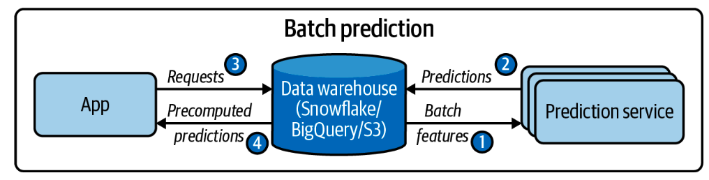
Fig. 50 A simplified architecture for batch prediction.#
Image Credits: Chip Huyen - Designing Machine Learning Systems
Example#
Batch serving is particularly suitable for tasks where the data doesn’t change rapidly and real-time predictions are not required. Here are a few examples:
User content recommendation: Recommending content to users based on their viewing history is a common use case for batch serving. For example, a streaming service like Netflix or Spotify could use batch serving to generate personalized content recommendations for all users overnight, based on their viewing or listening history up to the end of the previous day.
Predictive maintenance: Another use case is predicting equipment failures or maintenance needs based on sensor data. If the equipment doesn’t require real-time monitoring, the sensor data could be batch processed overnight to predict the probability of equipment failure in the next few days or weeks.
Marketing campaign planning: In marketing, batch serving could be used to segment the customer base and predict the expected response to different marketing campaigns. These predictions could be used to plan marketing activities for the next few days or weeks.
However, for new users who do not yet have a viewing history, the system might have to make generic recommendations based on their explicitly stated interests or demographic information. Also, for certain popular combinations of input features, caching could indeed be a valuable strategy to increase serving speed, even in a real-time serving setup. This is sometimes referred to as “hot data caching” or “frequently used data caching”.
Advantages#
The model generates and caches predictions, which enables very fast inference for users. This is because the model doesn’t have to process each input individually in real-time; instead, it retrieves the precomputed results from the database.
The model doesn’t need to be hosted as a live service since it’s never used in real-time. This can reduce the resource requirements and complexity of the deployment infrastructure.
Disadvantages#
The predictions can become stale or outdated if the user develops new interests that aren’t captured by the old data on which the current predictions are based. In other words, the model’s predictions won’t adapt quickly to changes in user behavior or other factors.
The input feature space must be finite because we need to generate all the predictions before they’re needed for real-time. This requirement limits the applicability of batch serving to certain use cases. For example, it might not be suitable for scenarios where the potential inputs are diverse or unpredictable, such as natural language processing tasks.
Setting up a Batch Serving System#
If you want to store predictions even when you don’t know in advance what input the users will provide, you can design your system to capture and store the predictions along with the corresponding user inputs. Here’s a general approach:
Set up a data storage system: Choose a suitable data storage solution such as a relational database, NoSQL database, or a data lake to store the predictions and associated user inputs. Select a storage solution that aligns with your system requirements in terms of scalability, query capabilities, and data retention policies.
Define a data schema: Determine the structure of the data you want to store. Define the necessary fields to capture the user inputs and the corresponding predictions. For example, you might include fields such as user ID, timestamp, input features, and predicted output.
Capture user inputs: Within your API or application, capture the user inputs as they interact with the system. Extract the relevant information from the user’s request, such as feature values or any contextual data you need for prediction.
Generate predictions: Pass the user inputs to your pre-trained model to generate predictions. Retrieve the output from the model for the given inputs.
Store the data: Once you have the user inputs and the corresponding predictions, store them in your chosen data storage system. Serialize the data in a format that can be stored, such as JSON or CSV, and save it in the appropriate database table or collection.
Retrieve predictions: At a later time, you can query the data storage system to retrieve and analyze the stored predictions. You can use SQL queries, NoSQL queries, or other methods supported by your chosen storage solution to filter, aggregate, or perform further analysis on the stored data.
By implementing this approach, you can store the predictions alongside the user inputs, enabling you to review and analyze the predictions later, gain insights, track performance, and potentially improve your models or system based on the collected data.
Real-Time Serving/Inference (Online with only Batch Features)#
Definition#
Real-time inference involves making predictions on the fly as soon as a request comes in. This approach is utilized when there’s a need for immediate prediction.
Visualization (Batch Features only)#
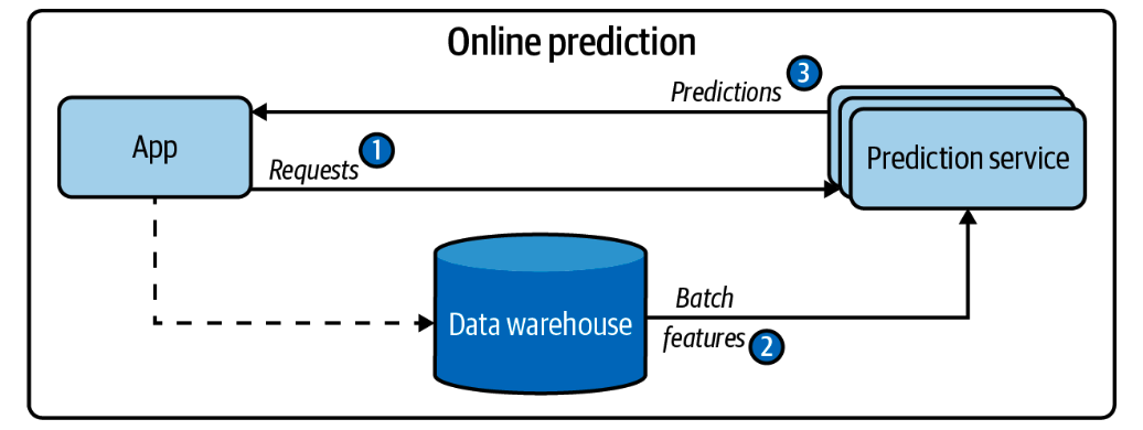
Fig. 51 A simplified architecture for online prediction that only uses batch features.#
Image Credits: Chip Huyen - Designing Machine Learning Systems
Say we have a recommender system recommending credit card (items) to users. The precomputer embeddings of credit card features may be static, but the user features may be different for each user. So, the user features are streaming features, and the credit card embeddings are batch features where we can store them in a database and retrieve them when needed to say, compute the cosine similarity between the user features and the credit card embeddings.
Visualization (Online Features)#
I do not have a diagram yet, but for instance, the users’ real-time activity/features are online features, and the credit card embeddings are batch features.
Example#
Fraud detection: A fraud detection system is a great example of a real-time inference application. In such a case, the model needs to evaluate transactions in real-time to prevent fraudulent activities.
Real-time personalization: In e-commerce, models might be used to personalize the shopping experience by recommending products or offers in real-time, based on the user’s current activity on the site.
Chatbots and virtual assistants: In conversational AI, models need to generate responses to user inputs in real-time.
Autocomplete: In search engines, models might be used to generate autocomplete suggestions in real-time as the user types in the search box.
Advantages#
Provides immediate predictions, which can enhance the user experience and provide immediate feedback.
More suitable for systems with an unbounded feature space, where inputs can change and evolve over time.
Disadvantages#
Requires more computational resources and infrastructure to handle real-time requests.
More complex to implement and manage due to the need to handle potentially high volumes of real-time requests.
Requires real-time monitoring to ensure the system is functioning correctly.
Streaming Inference#
Definition#
Streaming inference refers to the process of making predictions on a continuous stream of incoming data. This method is useful when the data is constantly updating and predictions need to be made as soon as the new data arrives.
Visualization#
Fig. 52 A simplified architecture for online prediction that uses both batch features and streaming features.#
Image Credits: Chip Huyen - Designing Machine Learning Systems
Example#
Streaming inference would be ideal for real-time monitoring of workplace safety based on continuous inputs from various sensors.
Imagine a manufacturing plant where safety is crucial. In this environment, there might be various sensors distributed throughout the facility, continuously monitoring factors like temperature, noise levels, vibration, toxic gas concentrations, and other environmental variables. There could also be cameras monitoring the physical activities of workers, ensuring that safety protocols are being followed.
A machine learning model could be set up to process this constant stream of sensor data in real time. Using streaming inference, the model would analyze each incoming piece of data as it arrives, looking for patterns or anomalies that might indicate a safety hazard.
For example, the model might predict a risk of equipment failure if it detects unusual vibration patterns from a specific machine. Or it might alert to a potential safety violation if it recognizes through video analysis that a worker isn’t wearing the required protective gear.
By using streaming inference in this way, the system can detect and respond to potential safety issues as soon as they arise, rather than waiting to analyze batches of data after the fact. This real-time response could prevent accidents, protect workers, and maintain productivity.
Advantages#
Can handle continuous streams of data and provide real-time predictions.
Particularly suitable for systems where the data is constantly updating and you need to make predictions as soon as new data arrives.
Disadvantages#
Requires infrastructure and resources to handle continuous streams of data.
More complex to implement and manage than batch or real-time inference.
Also requires real-time monitoring to ensure the system is functioning correctly.
Hybrid Serving#
However, online prediction and batch prediction don’t have to be mutually exclusive. One hybrid solution is that you precompute predictions for popular queries, then generate predictions online for less popular queries[1].
A real-world example of this hybrid solution could be an e-commerce recommendation system.
In this system, we could utilize embeddings to represent each product. An embedding is a way of representing a product in a high-dimensional space such that similar products are closer to each other. These embeddings can be pre-computed using historical data and used as batch features.
For popular products, you can precompute the “nearest neighbors” in the embedding space using batch prediction. This means that for each popular product, you identify a set of other products that are closest to it in the embedding space, i.e., the most similar products. These become your precomputed recommendations for that product.
Now, when a customer views a popular product, the system can instantly return the precomputed recommendations without needing to perform any online calculations. This approach helps to reduce the computation load and improve response times for the majority of customer interactions.
On the other hand, for less popular products or unique customer queries, you might not have precomputed recommendations. In this case, you need to perform online prediction. When a customer views a less common product, the system would calculate its position in the embedding space and find the nearest neighbors in real-time, thereby generating personalized recommendations.
In this way, embeddings can be used in both batch and online prediction settings, enabling a hybrid approach that balances computational efficiency with the ability to handle diverse customer needs.
On-Device Inference#
Definition#
On-device inference refers to a machine learning model making predictions on the device itself, rather than on a server. This method is often used when there’s a need for real-time predictions without relying on a stable internet connection.
Example#
Voice recognition models on smartphones, like Siri or Google Assistant, are classic examples of on-device inference. These models need to respond instantly to voice commands, and running the model on the device itself reduces latency.
Advantages#
Provides immediate predictions without needing a server or internet connection.
Can help to preserve user privacy as no data needs to be sent to a server.
Suitable for applications where the device might not always have a reliable internet connection.
Disadvantages#
Limited by the device’s computational resources, so models may need to be smaller and more efficient, potentially reducing their accuracy.
Can be more difficult to update and maintain models across multiple devices.
Implementing and managing models across a range of different device types and operating systems can add complexity.
Batch Processing does not mean Predicting all Possible Inputs in Advance#
There might be confusion around the batch processing and real-time processing.
In the context of machine learning model serving, batch processing doesn’t mean predicting all possible inputs in advance. Instead, it means that predictions for multiple inputs are made together in one batch, rather than one at a time.
For example, in a recommendation system, users’ activities might be collected over a day, and at the end of the day, recommendations for all users are generated together in a batch process and stored in a database. This doesn’t require knowing in advance what the users’ activities will be.
On the other hand, real-time processing means that the model makes a prediction for a single input immediately when it is received, without waiting for more inputs to process together in a batch.
The choice between batch processing and real-time processing often depends on the specific requirements of the use case.
Batch Processing: If the application does not require immediate responses, and computational resources are limited, batch processing can be a good choice. Batch processing is computationally efficient because it allows the machine learning system to process large amounts of data at once, taking full advantage of the parallel processing capabilities of modern hardware.
Real-time Processing: If the application requires immediate responses (e.g., fraud detection, autonomous vehicles, etc.), real-time processing is necessary. Real-time processing might be more computationally intensive since predictions need to be made immediately for each individual input.
So, when I mentioned the feature space (finite or unbounded) earlier, it was more about how difficult it might be to engineer features for batch or real-time processing. For finite feature spaces, feature engineering might be simpler, potentially making it easier to use batch processing. But for unbounded feature spaces, feature engineering can be more complex and computationally intensive, potentially making real-time processing more challenging.
But ultimately, the choice between batch and real-time depends more on the specific requirements of the application and the computational resources available.
From Batch Prediction to Online Prediction#
One thing that resonates well from Chip’s chapter on model serving[1] is that people coming from a traditional modelling or more academic background tend to be accustomed to online prediction as a natural way of transitioning from training to serving.
This is likely how most people interact with their models while prototyping. This is also likely easier to do for most companies when first deploying a model. You export your model, upload the exported model to Amazon SageMaker or Google App Engine, and get back an exposed endpoint. Now, if you send a request that contains an input to that endpoint, it will send back a prediction generated on that input[1].
In other words, I trained a nice model, I wrap it in a nice API like FastAPI, and I deploy it to a cloud service like AWS or GCP. Now, I can send requests to the API and get back predictions. This is online prediction. Rarely do we “precompute” predictions in advance and store them in a database for later use.
She listed out the pros and cons with online prediction, and I think it’s worth to go over her content in details.
References and Further Readings#
See Also
There’s many more topics to cover on model deployment and prediction service:
Unifying Batch Pipeline and Streaming Pipeline
Model Compression
Machine Learning on the Cloud and on the Edge
You can find more details in Chip’s book[1].
Huyen, Chip. “Chapter 7. Model Deployment and Prediction Service.” In Designing Machine Learning Systems: An Iterative Process for Production-Ready Applications, O’Reilly Media, Inc., 2022.